 |

|
| LastUpdate 6/22/2024 |
| �@My first encounter with computers was during a university lecture. It
was a lecture on how to write a programing language called "Fortran".
I remember punching holes in a peace of paper tape and letting a big computer
read the program I created. �@In my first year as a teacher , I encountered a computer called "NEC-PC9801" at the school where I worked. As a strage medium , I inserted a 5-inch floppy disk , which I think is quite large , into the main unit. �@By the way , the strage medium of the personal computer I purchased for home use was a casstte tape. It wasn't just for personal computers. It was for cassette tape recorders that are still around today for listening to and memorizing music. The boot program is also included in this cassette tape , and it takes about 5 minutes for the computer to start up. �@At that time , computers were machines for numerical processing and could not process mathematical formulas. However , computers now calculate not only numbers , but also formulas. If you use formula manipulation software , "organize formulas" , "expand" , "factorize" , "solve linear equation" , "solve quadratic equations" , "solve cubic equations" , "solve quartic equations" , " differentiate" , and "Integration" is easy for you to do. �@Three-dimensional graphs can be easily drawn using Maxima. By dragging the graph , you can freely change the viewing direction of the graph. �@Typical formula manipulation software includes (1) "Mathematica" , (2) "Maple" , and (3) "Maxima". While (1) , (2) are expensive , ranging from 200,000 yen to 300,000 yen , (3) "Maxima" is free software, so it is free. �@In addition , the source code of "Maxima "is open to the public (open source) , and all kinds of people around the world volunteer to participate in its development. "Maxima" is written in a programming language called "LISP". �@In addition , "wxMaxima 0.8.7"was used for the following examples. |
| �@�yExample 1�z�@Draw a graph of a 3D explicit function. �mMexican hat�n |
�m�P�nFunction expression �@�@�@ �m�Q�nInput formula �@plot3d(sin(sqrt(x^2+y^2))/sqrt(x^2+y^2),[x,-3*%pi,3*%pi],[y,-3*%pi,3*%pi],[plot_format,gnuplot],[grid,50,50]); �m�R�nDrawing result �@�@�@�@�@ 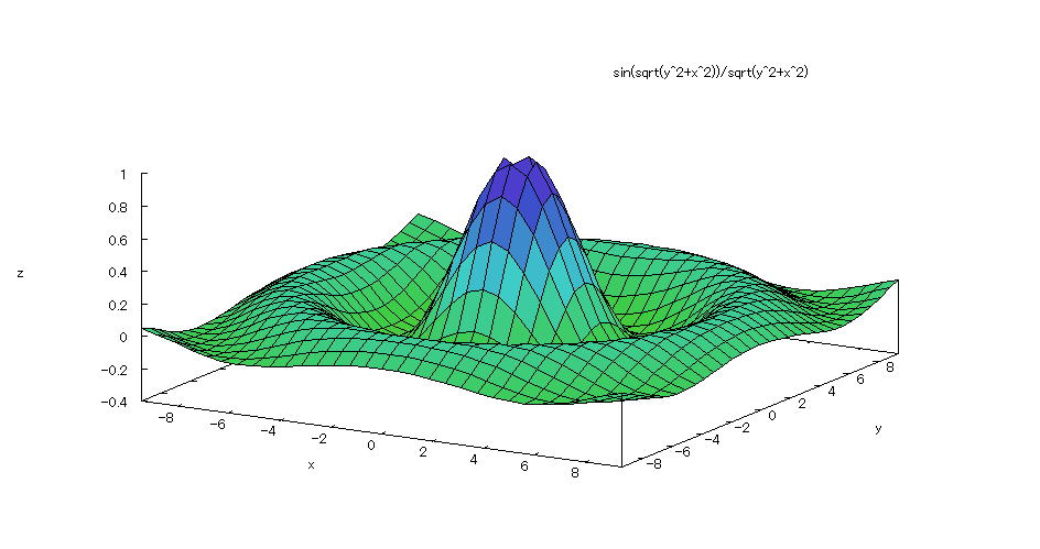 ��How to draw a graph�� �@As in the above input formula , enter all in half-width and press the Shift key and Enter key at the same time. �@ |
| �@�yExample 2�z�@Draw a graph of a 3D explicit function. �mCaldera shape�n |
�m�P�nFunction expression �@�@�@ �m�Q�nInput formula �@�@�@plot3d(exp(-(x^2+y^2)/2)*(x^2+y^2)/(2*%pi),[x,-2,2],[y,-2,2],[plot_format,gnuplot],[grid,50,50]); �m�R�nDrawing result �@�@�@�@�@ 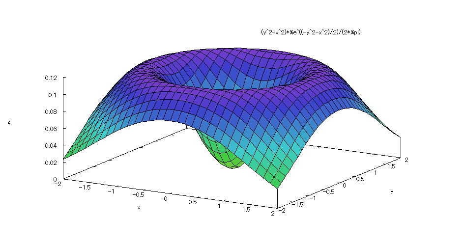 ��How to draw a graph�� �@ As in the above input formula , enter all in half-width and press the Shift key and Enter key at the same time. �@ |
| �@�yExample 3�z�@Draw a graph of a 3D explicit function. �mA slightly sunken saddle shape�n |
�m�P�nFunction expression �@�@�@ �m�Q�nInput formula �@�@�@plot3d(3*exp(-(x^2+y^2))*(2*x^2+y^2),[x,-2,2],[y,-2,2],[plot_format,gnuplot],[grid,50,50]); �m�R�nDrawing result �@�@�@�@�@ 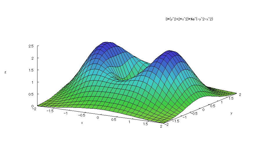 ��How to draw a graph�� �@ As in the above input formula , enter all in half-width and press the Shift key and Enter key at the same time. �@ |
| �@�yExample 4�z�@Draw a wireframe graph of a 3D implicit function. �mSphere�n |
�m�P�nFunction expression �@�@�@ �m�Q�nInput formula �@�@�@draw3d(implicit(x^2+y^2+z^2=1,x,-1,1,y,-1,1,z,-1,1)); �m�R�nDrawing result �@�@�@�@�@ 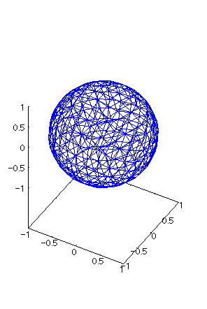 ��How to draw a graph�� �@First , input "load(draw)" and press the Shift key and Enter key at the same time to load the package. �@Next , as in the above input formula , enter all in half-width and press the Shift key and Enter key at the same time. �@ |
| �@�yExample 5�z�@Draw a graph of a 3D implicit function with hidden surface processing. �mSphere�n |
�m�P�nFunction expression �@�@�@ �m�Q�nInput formula �@�@�@draw3d(enhanced3d=true,implicit(x^2+y^2+z^2=1,x,-1,1,y,-1,1,z,-1,1)); �m�R�nDrawing result �@�@�@�@�@ 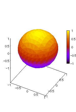 ��How to draw a graph�� �@First , input "load(draw)" and press the Shift key and Enter key at the same time to load the package. �@Next , as in the above input formula , enter all in half-width and press the Shift key and Enter key at the same time. �@ |
| �@�yExample 6�z Draw a graph of a 3D implicit function with hidden surface processing. �mHollow drum�n |
�m�P�nFunction expression �@�@�@ �m�Q�nInput formula �@�@�@draw3d(enhanced3d=true,implicit(x^2+y^2-z^2=1,x,-2,2,y,-2,2,z,-2,2)); �m�R�nDrawing result �@�@�@�@�@ 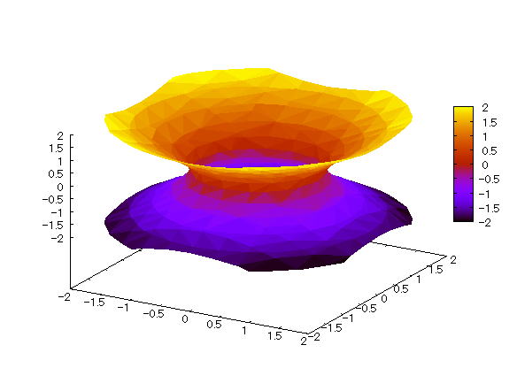 ��How to draw a graph�� �@First , input "load(draw)" and press the Shift key and Enter key at the same time to load the package. �@Next , as in the above input formula , enter all in half-width and press the Shift key and Enter key at the same time. �@ |
| �@�yExample 7�z Draw a graph of a 3D implicit function with hidden surface processing. �mSewer pipe joint�n |
�m�P�nFunction expression �@�@�@ �m�Q�nInput formula �@�@�@draw3d(enhanced3d=true,implicit((x^2-1)^2+(y^2-1)^2+(z^2-1)^2=1.5, x,-1,1,y,-1,1,z,-1,1)); �m�R�nDrawing result �@�@�@�@�@ 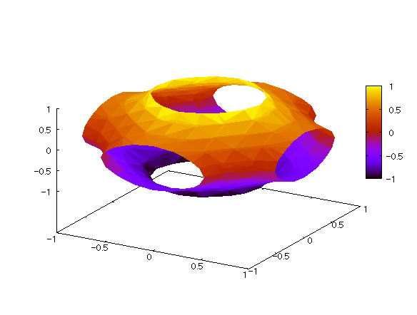 ��How to draw a graph�� �@First , input "load(draw)" and press the Shift key and Enter key at the same time to load the package. �@Next , as in the above input formula , enter all in half-width and press the Shift key and Enter key at the same time. �@ |
| �@�yExample 8�z�@Draw a graph of a 3D implicit function with hidden surface processing. �ma cell with nucleus in the center�n |
�m�P�nFunction expression �@�@�@������(���{�ӂ�)�{������(���|�ӂ�) �{������(���{�ӂ�)�{������(���|�ӂ�)�{������(���{�ӂ�)�{������(���|�ӂ�)���Q �@�@�@�@�@�@�@�@�@�@�@�@�@�@�@�@�@�@�@�@�@�@�@�@�@�@�@�@�@�@�@�iHowever , �� represents the golden ratio.�j �m�Q�nInput formula �@�@�@draw3d(enhanced3d=true,implicit(cos(x+%phi*y)+cos(x-%phi*y)+cos(y+%phi*z) �@�@�@�@�@�@�@�@�@�@�@�@�@�@�@�@�@+cos(y-%phi*z)+cos(z+%phi*x)+cos(z-%phi*x)=2,x,-4,4,y,-4,4,z,-4,4)); �m�R�nDrawing result �@�@�@�@�@ 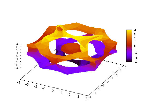 ��How to draw a graph�� �@First , input "load(draw)" and press the Shift key and Enter key at the same time to load the package. �@Next , as in the above input formula , enter all in half-width and press the Shift key and Enter key at the same time. �@ |
| �@�yExample 9�z�@Draw a graph of a 3D parameter. �mSphere�n |
�m�P�nFunction expression �@�@�@�������������E�������� �@�@�@�������������E�������� �@�@�@�������������@�@�@�@�@�@�@�@�i�O�������Q�j �i�O�������j �m�Q�nInput formula �@�@�@plot3d([cos(s)*cos(t),cos(s)*sin(t),sin(s)],[s,0,2*%pi],[t,0,%pi]); �m�R�nDrawing result �@�@�@�@�@ 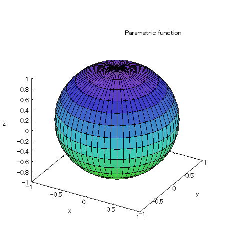 ��How to draw a graph�� �@As in the above input formula , enter all in half-width and press the Shift key and Enter key at the same time. �@ |
| �@�yExample 10�z�@Draw a graph of a 3D parameter. �mDonut shape�itorus�j�n |
�m�P�nFunction expression �@�@�@����(�T�{�Q��������)�������� �@�@�@����(�T�{�Q��������)�������� �@�@�@�����Q�������� �@�@�@�@�@�@�@�@�@�@�@�i�O�������Q�j �i�O�������Q�j �m�Q�nInput formula �@�@�@plot3d([(5+2*cos(s))*cos(t),(5+2*cos(s))*sin(t),2*sin(s)],[s,0,2*%pi],[t,0,2*%pi]); �m�R�nDrawing result �@�@�@�@�@ 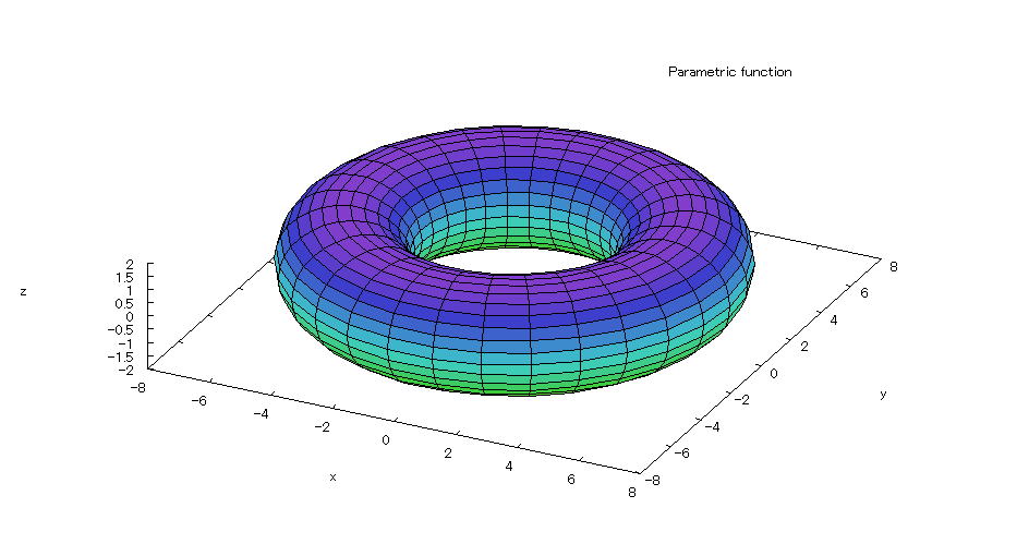 ��How to draw a graph�� �@ As in the above input formula , enter all in half-width and press the Shift key and Enter key at the same time. �@ |
| �@�yExample 11�z�@Draw a graph of a 3D parameter �mSpring type�n |
�m�P�nFunction expression �@�@�@����(�T�{��������)�������� �@�@�@����(�T�{��������)�������� �@�@�@�������������{�O�D�U�� �@�@�@�@�@�i�O�������Q�j �i�O�������V�j �m�Q�nInput formula �@�@�@plot3d([(5+cos(s))*cos(t),(5+cos(s))*sin(t),sin(s)+0.6*t],[s,0,2*%pi],[t,0,7*%pi]); �m�R�nDrawing result �@�@�@�@�@ 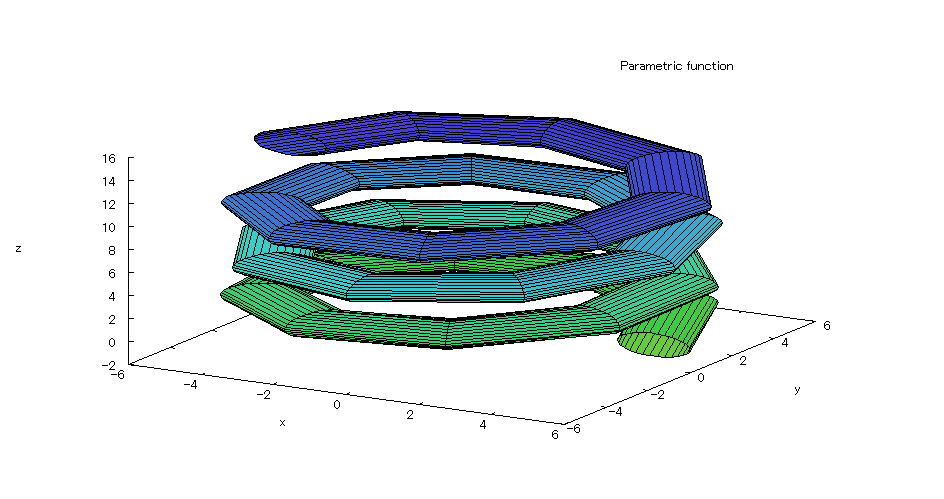 ��How to draw a graph�� �@As in the above input formula , enter all in half-width and press the Shift key and Enter key at the same time. �@ |
| �@�yExample 12�z�@Draw a graph of a 3D parameter. �mMobius strip�n |
�m�P�nFunction expression �@�@�@ �@�@�@ �@�@�@ �m�Q�nInput formula �@�@�@plot3d([cos(s)*(3+t*cos(s/2)),sin(s)*(3+t*cos(s/2)),t*sin(s/2)],[s,0-%pi,%pi],[t,-1,1]); �m�R�nDrawing result �@�@�@�@�@ 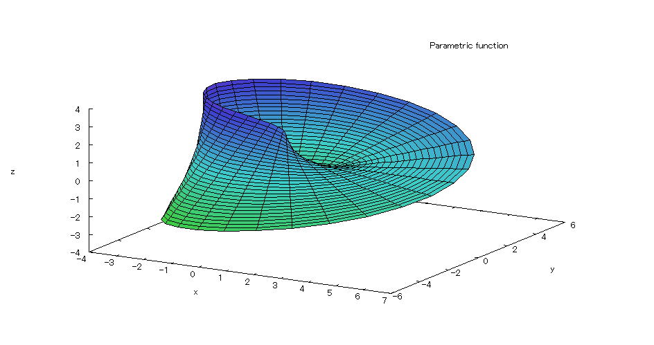 ��How to draw a graph�� �@As in the above input formula , enter all in half-width and press the Shift key and Enter key at the same time. �@ |
| �@�yExample 13�z�@Draw a graph of a 3D parameter. �mKlein's jar�n |
�m�P�nFunction expression �@�@�@ �@�@�@ �@�@�@ �@�@�@�@�@�@�@�@�@�@�@�@�@�@�@�@�@�@�@�@�@�@�@�@�@�@�@�@�@�@�@�@�@�@�@�@�@�@�@�@�i�|�������j �i�|�������j �m�Q�nInput formula �@�@�@plot3d([5*cos(s)*(cos(s/2)*cos(t)+sin(s/2)*sin(2*t)+3)-10, �@�@�@�@-5*sin(s)*(cos(s/2)*cos(t)+sin(s/2)*sin(2*t)+3.0),5*(-sin(s/2)*cos(t)+cos(s/2)*sin(2*t))], �@�@�@�@�@[s,-%pi,%pi],[t,-%pi,%pi]); �m�R�nDrawing result �@�@�@�@�@ 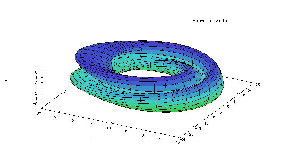 ��How to draw a graph�� �@As in the above input formula , enter all in half-width and press the Shift key and Enter key at the same time. �@ |
| �@�yExample14�z�@Draw a graph of a 2D explicit function. �mQuadratic function�n |
�m�P�nFunction expression �@�@�@ �m�Q�nInput formula �@�@�@ plot2d(3*x^2-1,[x,-2,2]); �m�R�nDrawing result �@�@�@�@�@ 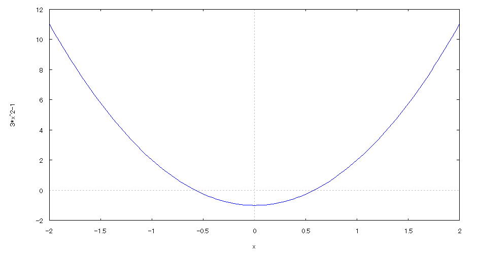 ��How to draw a graph�� �@As in the above input formula , enter all in half-width and press the Shift key and Enter key at the same time. �@ |
| �@�yExample 15�z�@Draw a graph of a 2D explicit function. �mExpotential�ETrigonometric function�n |
�m�P�nFunction expression �@�@�@�@ �m�Q�nInput formula �@�@�@ plot2d(exp(x)*sin(7*x),[x,0,20]); �m�R�nDrawing result �@�@�@�@�@ 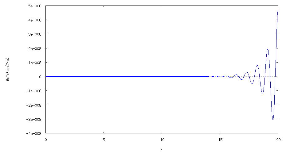 ��How to draw a graph�� �@As in the above input formula , enter all in half-width and press the Shift key and Enter key at the same time. �@ |
| �@�yExample 16�z�@Draw a graph of a 2D explicit function. �mDraw multiple graphs simultaneously�n |
�m�P�nFunction expression �@�@�@�@�@�������������A�����������Q���A�����������R���@�@�@�i�O�������Q�j �m�Q�nInput formula �@�@�@ plot2d([sin(x),sin(2*x),sin(3*x)],[x,0,2*%pi]); �m�R�nDrawing result �@�@�@�@�@ 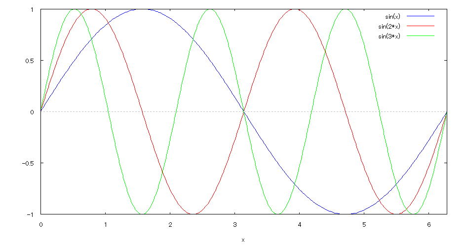 ��How to draw a graph�� �@As in the above input formula , enter all in half-width and press the Shift key and Enter key at the same time. �@ |
| �@�yExample 17�z�@Draw a graph of a 2D implicit function. �mCircle�n |
�m�P�nFunction expression �@�@�@�@ �m�Q�nInput formula �@�@�@ implicit_plot(x^2+y^2=1,[x,-2,2],[y,-2,2]); �m�R�nDrawing result �@�@�@�@�@ 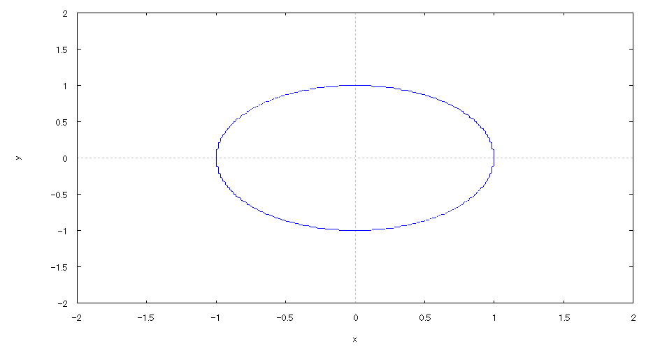 ��How to draw a graph�� �@First , input "load(implicitplot)" and press the Shift key and Enter key at the same time to load the package. �@Next , as in the above input formula , enter all in half-width and press the Shift key and Enter key at the same time. �@ |
| �@�yExample 18�z�@Draw a graph of a 2D implicit function. �mFour leaf clover�n |
�m�P�nFunction expression �@�@�@�@ �@�@�@ �m�Q�nInput formula �@�@�@ implicit_plot((x^2+y^2)^4-(x^2-y^2)^2=0,[x,-2,2],[y,-2,2]); �m�R�nDrawing result �@�@�@�@�@ 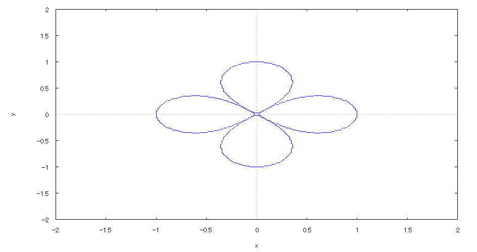 ��How to draw a graph�� �@First , input "load(implicitplot)" and press the Shift key and Enter key at the same time to load the package. �@Next , as in the above input formula , enter all in half-width and press the Shift key and Enter key at the same time. �@ |
| �@�yExample 19�z�@Draw a graph of a 2D implicit function. �mCircle and Four leaf clover�n |
�m�P�nFunction expression �@�@�@�@ �@�@�@�@ �m�Q�nInput formula �@�@�@ plot2d([x^2+y^2=1,(x^2+y^2)^4-(x^2-y^2)^2=0],[x,-2,2],[y,-2,2]); �m�R�nDrawing result �@�@�@�@�@ 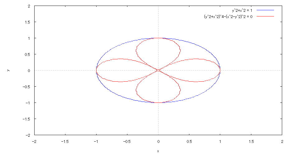 ��How to draw a graph�� �@First , input "load(implicitplot)" and press the Shift key and Enter key at the same time to load the package. �@Next , as in the above input formula , enter all in half-width and press the Shift key and Enter key at the same time. �@ |
| �@�yExample 20�z�@Draw a graph of a 2D parameter. �m�� shape�n |
�m�P�nFunction expression �@�@�@�@������������ �@�@�@�@�����������Q�� �@�i�O�������Q�j �P�O�O divisions �m�Q�nInput formula �@�@�@ plot2d([parametric,cos(t),sin(2*t)],[t,0,2*%pi],[nticks,100]); �m�R�nDrawing result �@�@�@�@�@ 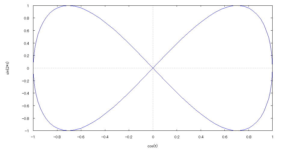 ��How to draw a graph�� �@As in the above input formula , enter all in half-width and press the Shift key and Enter key at the same time. �@ |
| �@�yExample 21�z�@Draw a graph of a 2D parameter. �mChrysanthemum petal shape�n |
�m�P�nFunction expression �@�@�@�@�����S�������S���������� �@�@�@�@�����S�������S���������� �@�i�O�������Q�j�@ �S�O�O divisions �m�Q�nInput formula �@�@�@ plot2d([parametric,4*sin(4*t)*cos(t),4*sin(4*t)*sin(t)],[t,0,2*%pi],[nticks,400]); �m�R�nDrawing result �@�@�@�@�@ 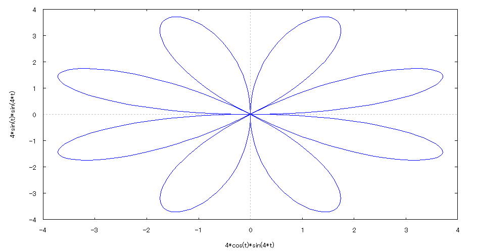 ��How to draw a graph�� �@As in the above input formula , enter all in half-width and press the Shift key and Enter key at the same time. �@ |
| �@�yExample 22�z�@Draw a graph of a 2D parameter. �mSwirl shape�n |
�m�P�nFunction expression �@�@�@�@���������������@�@�@�@ �@ �@�@�@�@�������������� �@�@�@�@�@ �m�Q�nInput formula �@�@�@ plot2d([parametric,t*cos(t),t*sin(t)],[t,0,35*%pi/2],[nticks,500]); �m�R�nDrawing result �@�@�@�@�@ 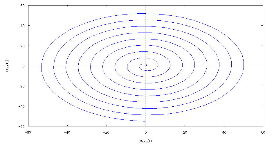 ��How to draw a graph�� �@As in the above input formula , enter all in half-width and press the Shift key and Enter key at the same time. �@ |
| �@�yExample 23�z�@Draw a graph of a 2D parameter. �mHeart shape�n |
�m�P�nFunction expression �@�@�@�@����(�P�{��������)�������� �@�@�@�@����(�P�{��������)�������� �@�@�i�O�������Q�j�@ �P�O�O divisions �m�Q�nInput formula �@�@�@ plot2d([parametric,(1+cos(t))*cos(t),(1+cos(t))*sin(t)],[t,0,2*%pi],[nticks,100]); �m�R�nDrawing result �@�@�@�@�@ 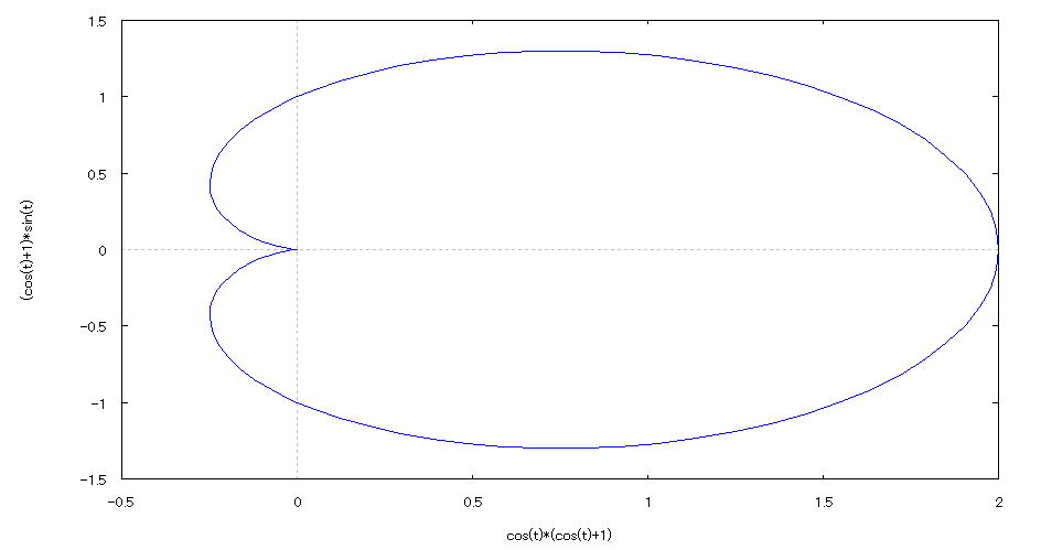 ��How to draw a graph�� �@As in the above input formula , enter all in half-width and press the Shift key and Enter key at the same time. �@ |
| �@�yExample 24�z�@Draw a wireframe graph of a 3D implicit function. �mellipsoid�n |
�m�P�nFunction expression �@�@�@ �m�Q�nInput formula �@�@�@draw3d(implicit(x^2/1^2+y^2/2^2+z^2/3^2=1,x,-1,1,y,-2,2,z,-3,3)); �@�@�@ �m�R�nDrawing result �@�@�@�@�@ 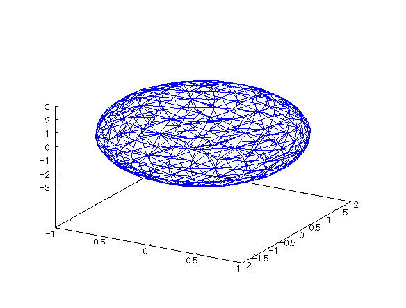 ��How to draw a graph�� �@First , input "load(draw)" and press the Shift key and Enter key at the same time to load the package. �@Next , as in the above input formula , enter all in half-width and press the Shift key and Enter key at the same time. �@ |
| �@�yExample 25�z�@Draw a wireframe graph of a 3D implicit function. �mSingle leaf hyperbola�n |
�m�P�nFunction expression �@�@�@ �m�Q�nInput formula �@�@�@draw3d(implicit(x^2/1^2+y^2/2^2-z^2/3^2=1,x,-7,7,y,-7,7,z,-7,7)); �@�@�@ �m�R�nDrawing result �@�@�@�@�@ 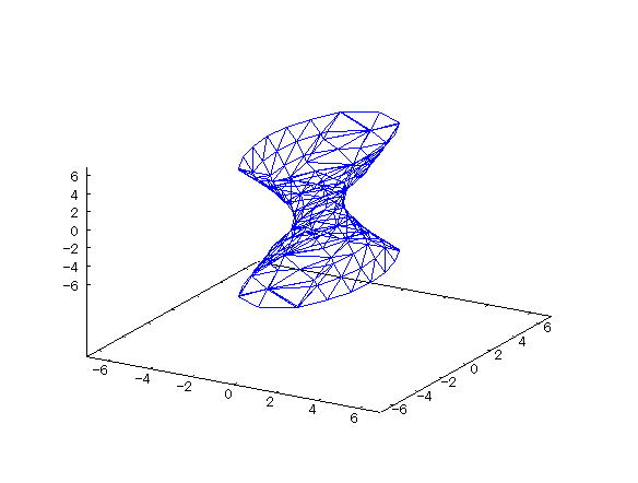 ��How to draw a graph�� �@First , input "load(draw)" and press the Shift key and Enter key at the same time to load the package. �@Next , as in the above input formula , enter all in half-width and press the Shift key and Enter key at the same time. �@ |
| �@�yExample 26�z�@Draw a wireframe graph of a 3D implicit function. �mBilobal hyperbola�n |
�m�P�nFunction expression �@�@�@ �m�Q�nInput formula �@�@�@draw3d(implicit(x^2/1^2-y^2/2^2-z^2/3^2=1,x,-2,2,y,-4,4,z,-8,8)); �@�@�@ �m�R�nDrawing result �@�@�@�@�@ 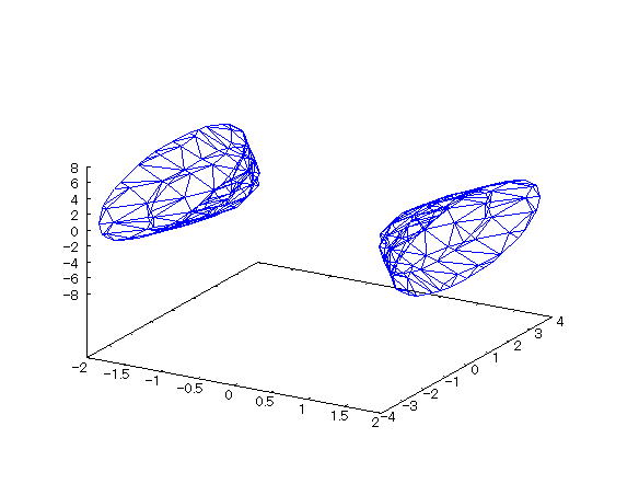 ��How to draw a graph�� �@First , input "load(draw)" and press the Shift key and Enter key at the same time to load the package. �@Next , as in the above input formula , enter all in half-width and press the Shift key and Enter key at the same time. �@ |
| �@�yExample 27�z�@Draw a wireframe graph of a 3D implicit function. �mElliptical paraboloid�n |
�m�P�nFunction expression �@�@�@ �m�Q�nInput formula �@�@�@draw3d(implicit(x^2/1^2+y^2/2^2=1/20*z,x,-1,1,y,-2,2,z,0,20)); �@�@�@ �m�R�nDrawing result �@�@�@�@�@ 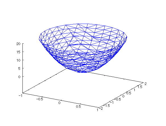 ��How to draw a graph�� �@First , input "load(draw)" and press the Shift key and Enter key at the same time to load the package. �@Next , as in the above input formula , enter all in half-width and press the Shift key and Enter key at the same time. �@ |
| �@�yExample 28�z�@Draw a wireframe graph of a 3D implicit function. �mHyperbolic paraboloid�n |
�m�P�nFunction expression �@�@�@ �m�Q�nInput formula �@�@�@draw3d(implicit(x^2/1^2-y^2/2^2=1/2*z,x,-2,2,y,-3,3,z,-4,4)); �@�@�@ �m�R�nDrawing result �@�@�@�@�@ 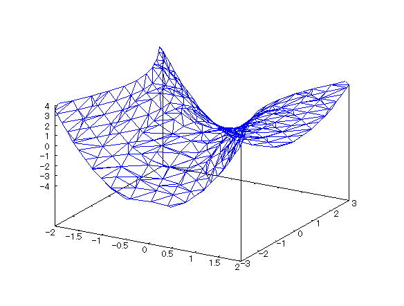 ��How to draw a graph�� �@First , input "load(draw)" and press the Shift key and Enter key at the same time to load the package. �@Next , as in the above input formula , enter all in half-width and press the Shift key and Enter key at the same time. �@ |
| �@�yExample 29�z�@Draw a wireframe graph of a 3D implicit function. �mElliptical cylinder�n |
�m�P�nFunction expression �@�@�@ �m�Q�nInput formula �@�@�@draw3d(implicit(x^2/1^2+y^2/2^2=1,x,-2,2,y,-2,2,z,-10,10)); �@�@�@ �m�R�nDrawing result �@�@�@�@�@ 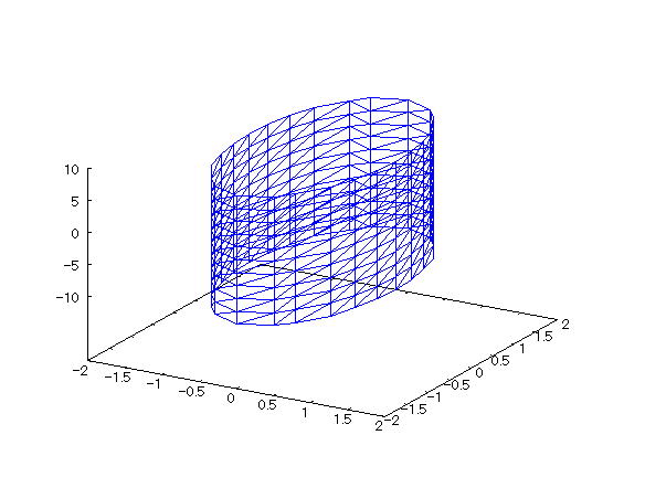 ��How to draw a graph�� �@First , input "load(draw)" and press the Shift key and Enter key at the same time to load the package. �@Next , as in the above input formula , enter all in half-width and press the Shift key and Enter key at the same time. �@ |
| �@�yExample 30�z�@Draw a wireframe graph of a 3D implicit function. �mHyperbolic column�n |
�m�P�nFunction expression �@�@�@ �m�Q�nInput formula �@�@�@draw3d(implicit(x^2/2^2-y^2/3^2=1,x,-10,10,y,-10,10,z,-20,20)); �@�@�@ �m�R�nDrawing result �@�@�@�@�@ 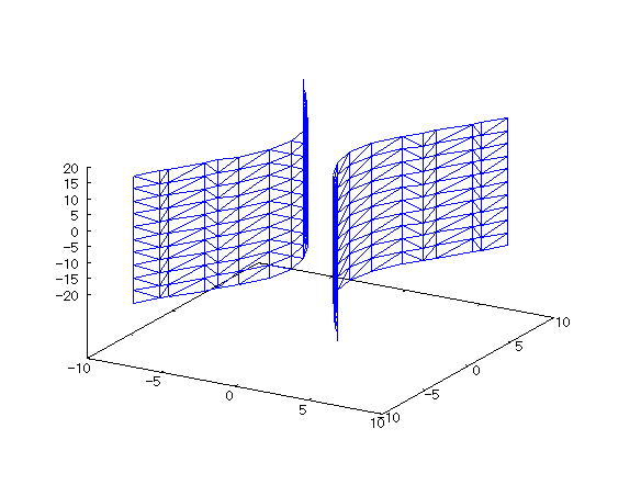 ��How to draw a graph�� �@First , input "load(draw)" and press the Shift key and Enter key at the same time to load the package. �@Next , as in the above input formula , enter all in half-width and press the Shift key and Enter key at the same time. �@ |
| �@�yExample 31�z�@Draw a wireframe graph of a 3D implicit function. �mParabolic column�n |
�m�P�nFunction expression �@�@�@ �m�Q�nInput formula �@�@�@draw3d(implicit(x^2=y,x,-5,5,y,0,25,z,-20,20)); �@�@�@ �m�R�nDrawing result �@�@�@�@�@ 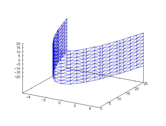 ��How to draw a graph�� �@First , input "load(draw)" and press the Shift key and Enter key at the same time to load the package. �@Next , as in the above input formula , enter all in half-width and press the Shift key and Enter key at the same time. �@ |
| �@�yExample 32�z�@Draw a graph of a 2D explicit function. �mMake it easier to see by specifying the range of y values�n |
�m�P�nFunction expression �@�@�@ �m�Q�nInput formula �@�@�@plot2d((x^3+2*x^2-4*x-3)/(x+1),[x,-3,3],[y,-10,10]); �@�@�@ �m�R�nDrawing result �@�@�@�@�@ 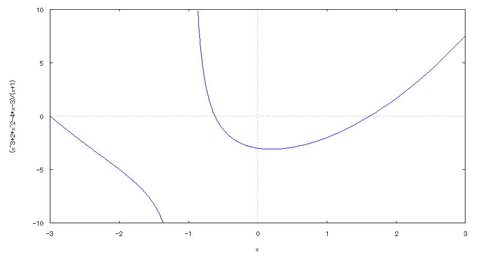 ��How to draw a graph�� �@As in the above input formula , enter all in half-width and press the Shift key and Enter key at the same time. �@ |
| �@�yExample 33�z�@Draw a graph of a 2D explicit function. �mDisplay multiple graphs simultaneously�n |
�m�P�nFunction expression �@�@�@ �m�Q�nInput formula �@�@�@plot2d([exp(-2*x),exp(x),1],[x,-2,2],[y,0,10]); �@�@�@ �m�R�nDrawing result �@�@�@�@�@ 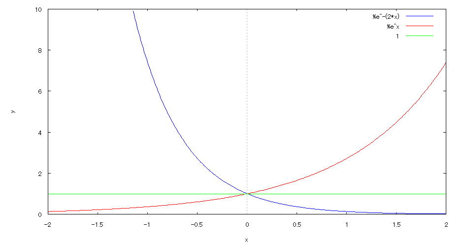 ��How to draw a graph�� �@As in the above input formula , enter all in half-width and press the Shift key and Enter key at the same time. �@ |
| �@�yExample 34�z�@Draw a graph of a 2D explicit function. �mFind the number of real solutions to an equation�n |
�m�P�nEquation �@�@�@ �m�Q�nInput formula �@�@�@plot2d([x/8,cos(x)],[x,-15,15],[y,-2,2]); �@�@�@ �m�R�nDrawing result �@�@�@�@�@ 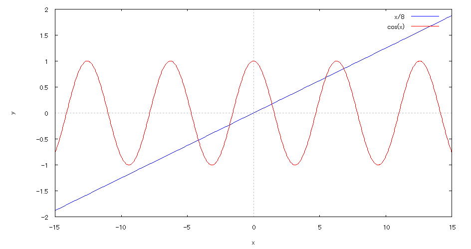 ��How to draw a graph�� �@As in the above input formula , enter all in half-width and press the Shift key and Enter key at the same time. �@Since there are 5 intersections , we know that the equation has 5 real solutions. �@ |
| �@�yExample 35�z�@Draw a graph of a 2D parameter. �mSpecify the number of divisions�n |
�m�P�nFunction expression �@�@�@ �m�Q�nInput formula �@�@�@plot2d([parametric,3*cos(t)+cos(13*t),3*sin(t)+sin(13*t)],[t,0,2*%pi],[nticks,300]); �@�@�@ �m�R�nDrawing result �@�@�@�@�@ 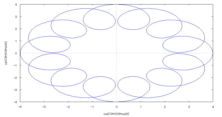 ��How to draw a graph�� �@As in the above input formula , enter all in half-width and press the Shift key and Enter key at the same time. �@ |
| �@�yExample 36�z�@Draw a graph of a 2D parameter. �mLissajous curve�n |
�m�P�nFunction expression �@�@�@ �m�Q�nInput formula �@�@�@plot2d([parametric,cos(7*t),sin(4*t)],[t,0,2*%pi],[nticks,300]); �@�@�@ �m�R�nDrawing result �@�@�@�@�@ 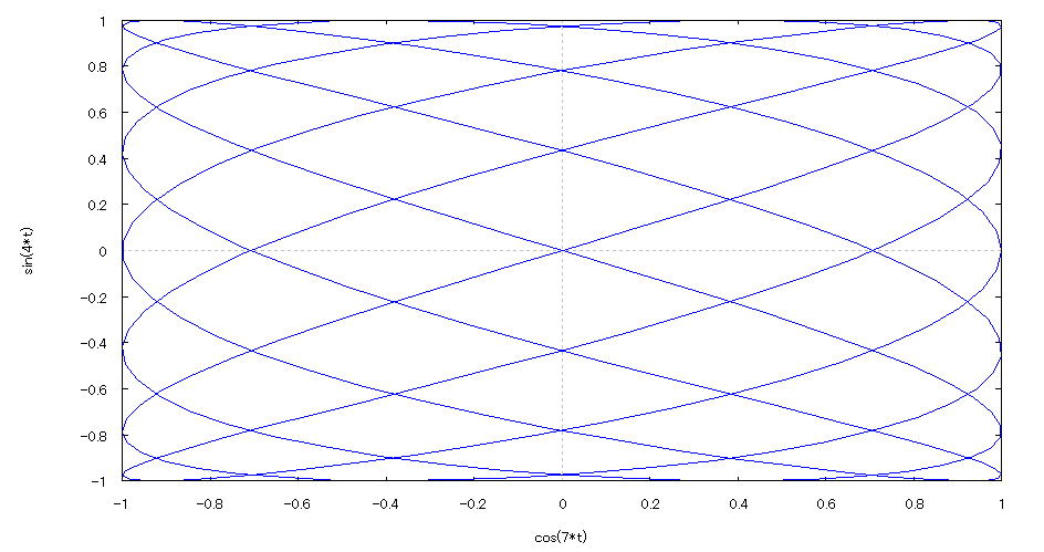 ��How to draw a graph�� �@As in the above input formula , enter all in half-width and press the Shift key and Enter key at the same time. �@ |
| �@�yExample 37�z�@Draw a graph of a 2D parameter. �mBernoulli's lemniscate curve�n |
�m�P�nFunction expression �@�@�@ �m�Q�nInput formula �@�@�@plot2d([parametric,cos(t)/(1+sin(t)^2),sin(t)*cos(t)/(1+sin(t)^2)],[t,0,2*%pi],[nticks,300]); �@�@�@ �m�R�nDrawing result �@�@�@�@�@ 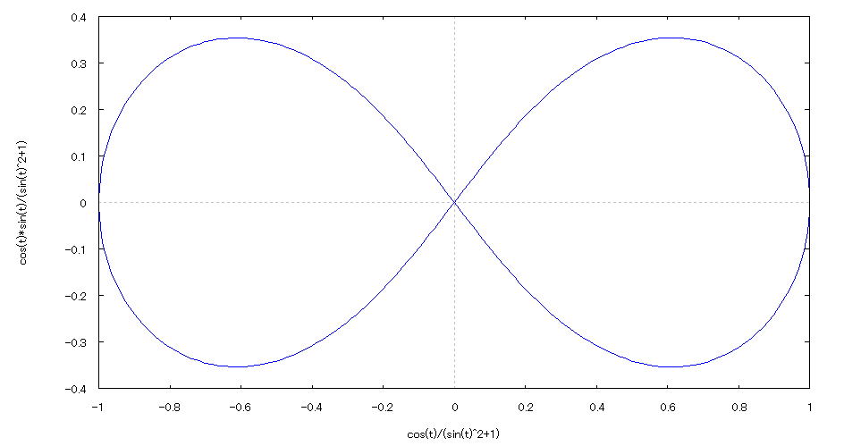 ��How to draw a graph�� �@As in the above input formula , enter all in half-width and press the Shift key and Enter key at the same time. �@ |
| �@�yExample 38�z�@Draw a graph of a 3D explicit function. �mDo not specify the number of devisions�n |
�m�P�nFunction expression �@�@�@ �m�Q�nInput formula �@�@�@plot3d(exp(-sqrt(x^2+y^2)/2)*cos(%pi*sqrt(x^2+y^2)),[x,-4,4],[y,-4,4]); �@�@�@ �m�R�nDrawing result �@�@�@�@�@ 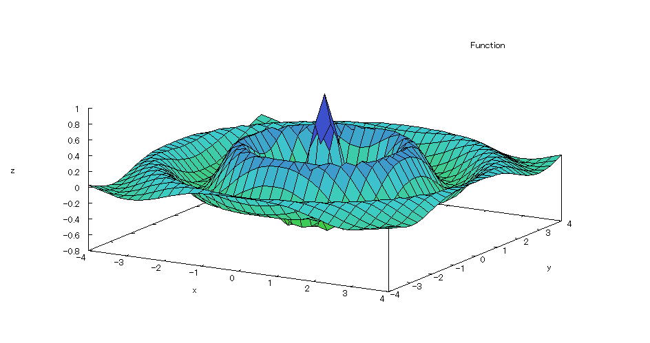 ��How to draw a graph�� �@As in the above input formula , enter all in half-width and press the Shift key and Enter key at the same time. �@ |
| �@�yExample 39�z�@Draw a graph of a 3D explicit function. �mShark minimal surface�n |
�m�P�nFunction expression �@�@�@ �m�Q�nInput formula �@�@�@plot3d(log(cos(x)/cos(y)),[x,-%pi/2,%pi/2],[y,-%pi/2,%pi/2]); �@�@�@ �m�R�nDrawing result �@�@�@�@�@ 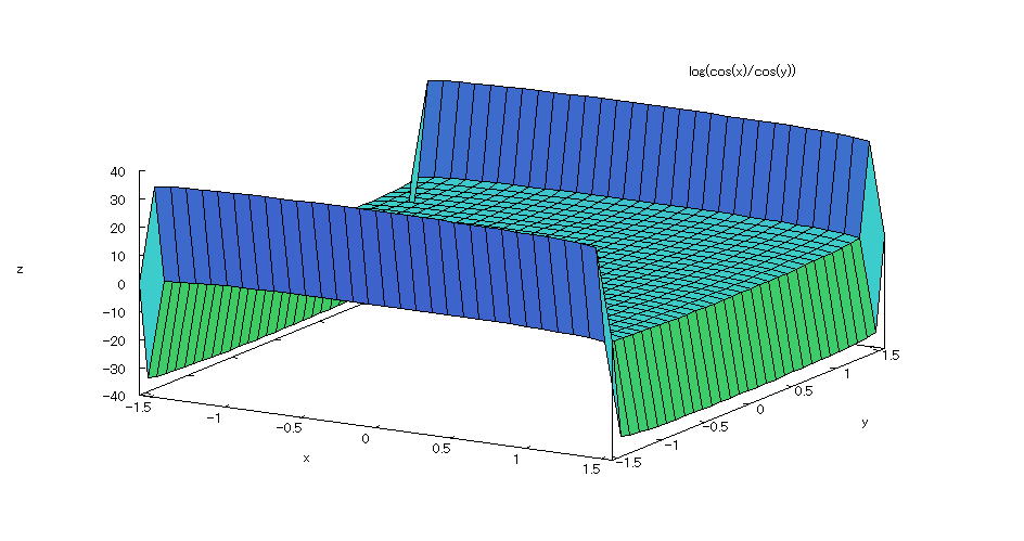 ��How to draw a graph�� �@As in the above input formula , enter all in half-width and press the Shift key and Enter key at the same time. �@ |
| �@�yExample 40�z�@Draw a graph of a 3D explicit function. �mDefine and draw a function�n |
�m�P�nFunction expression �@�@�@�@�@ 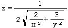 �@�@�@�i�O�������Q�C�O�������Q�j �@�@�@�i�O�������Q�C�O�������Q�j�m�Q�nInput formula �@�@�@u(a,x,y,p,q,r):=a*(p*x^(-r)+q*y^(-r))^(-1/r); �@�@�@plot3d(u(2,x,y,2,3,2),[x,0.01,2],[y,0.01,2]); �@�@�@ �m�R�nDrawing result �@�@�@�@�@ 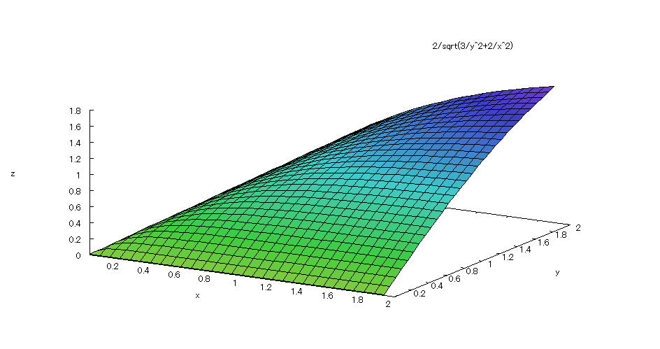 ��How to draw a graph�� �@First , enter the first line of the above input express in half-width , and press the Shift key and Enter key at the same time. �@Next , enter the second line in half-width and press the Shift key and Enter key at the same time. �@ |
| �@�yExample 41�z�@Draw a graph of a 3D parameter. �mTorus�n |
�m�P�nFunction expression �@�@�@ �@�@�@ �@�O�������Q�A�O�������Q�� �m�Q�nInput formula �@�@�@plot3d([cos(s)*(3+cos(t)),sin(s)*(3+cos(t)),sin(t)],[s,0,2*%pi],[t,0,2*%pi]); �@�@�@ �m�R�nDrawing result �@�@�@�@�@ 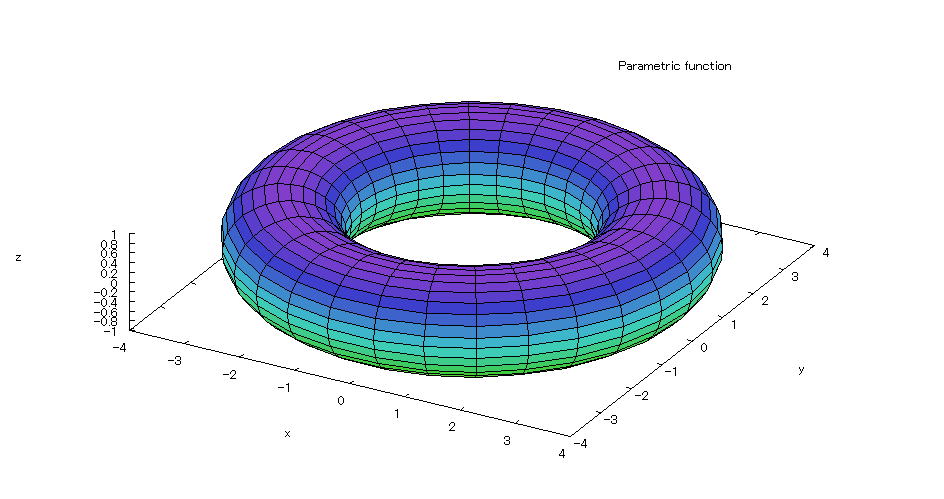 ��How to draw a graph�� �@As in the above input formula , enter all in half-width and press the Shift key and Enter key at the same time. �@ |
| �@�yExample 42�z�@Draw a graph of a 3D parameter. �mAsteroidal sphere�n |
�m�P�nFunction expression �@�@�@ �@�@�@ �@�O�������Q�A�O�������Q�� �m�Q�nInput formula �@�@�@plot3d([cos(s)^3*cos(t)^3,sin(s)^3*cos(t)^3,sin(t)^3],[s,0,2*%pi],[t,0,2*%pi]); �@�@�@ �m�R�nDrawing result �@�@�@�@�@ 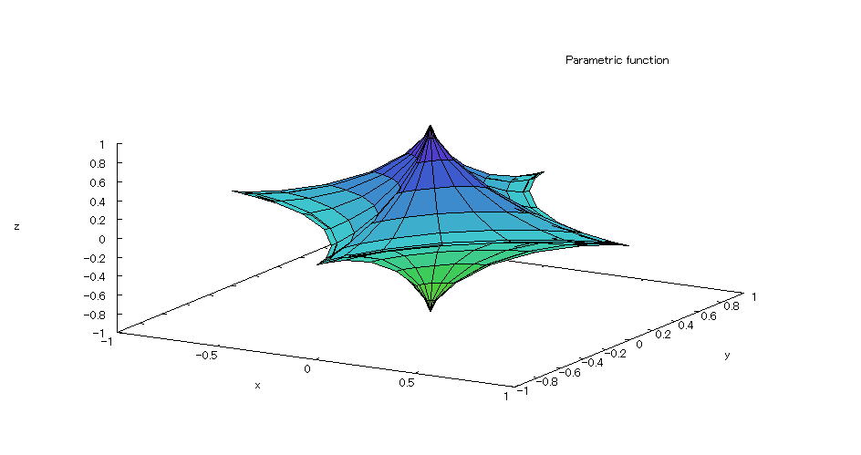 ��How to draw a graph�� �@As in the above input formula , enter all in half-width and press the Shift key and Enter key at the same time. �@ |
| �@�yExample 43�z�@Draw a graph of a 3D parameter. �mHenneberg Minimal Surface�n |
�m�P�nFunction expression �@�@�@�@ �@�@�@�@ �@�@�@�@ �@�@�@ �@�O�D�R�������O�D�X�@�A�@�O�������Q�� �m�Q�nInput formula �@�@�@plot3d([2*sinh(s)*cos(t)-(2/3)*sinh(3*s)*cos(3*t),2*sinh(s)*sin(t)-(2/3)*sinh(3*s) �@�@�@�@�@�@�@�@�@�@�@�@�@�@�@�@�@�@*sin(3*t),2*cosh(2*s)*cos(2*t)],[s,0.3,0.9],[t,0,2*%pi],[grid,4,72]); �m�R�nDrawing result �@�@�@�@�@ 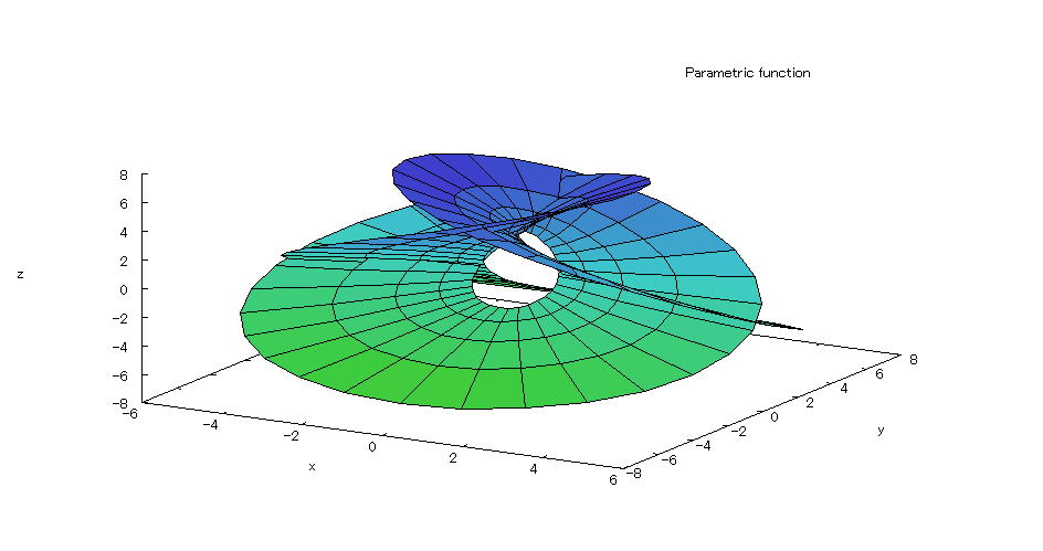 ��How to draw a graph�� �@As in the above input formula , enter all in half-width and press the Shift key and Enter key at the same time. �@ |
| �@�yExample 44�z�@Draw a graph of a 2D explicit function. �mMake it easier to see by specifying the range of y-axis values�n |
�m�P�nFunction expression �@�@�@�@ �m�Q�nInput formula �@�@�@plot2d(1/(x-1)+1,[x,-5,5],[y,-5,5]); �m�R�nDrawing result �@�@�@�@�@ 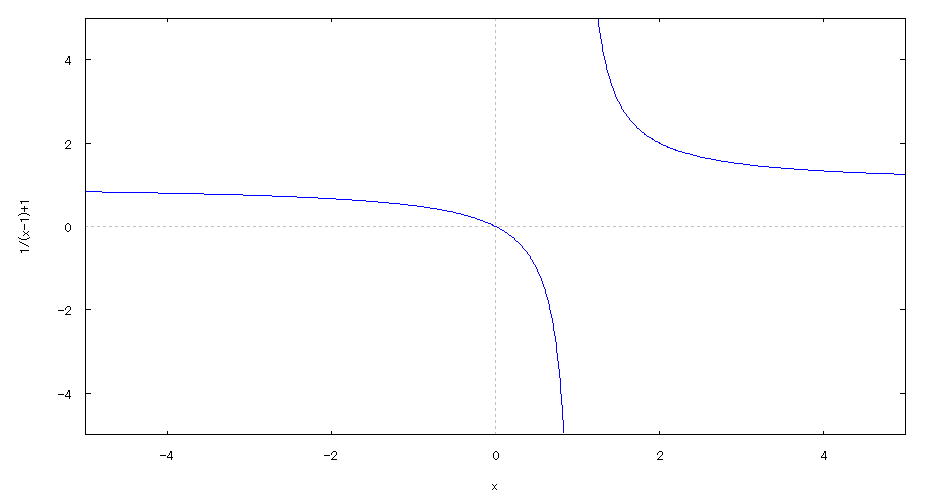 ��How to draw a graph�� �@As in the above input formula , enter all in half-width and press the Shift key and Enter key at the same time. �@ |
| �@�yExample 45�z�@Draw a graph of a 2D explicit function. �mCompare with the Taylor expansion graph of the approximation formula�n |
�m�P�nFunction expression �@�@�@�@ �m�Q�nInput formula �@�@�@plot2d([cos(x),1-x^2/2+x^4/24-x^6/720,1-x^2/2+x^4/24-x^6/720+x^8/40320, �@�@�@�@�@�@�@�@1-x^2/2+x^4/24-x^6/720+x^8/40320-x^10/3628800],[x,-2*%pi,2*%pi],[y,-5,5]); �m�R�nDrawing result �@�@�@�@�@ 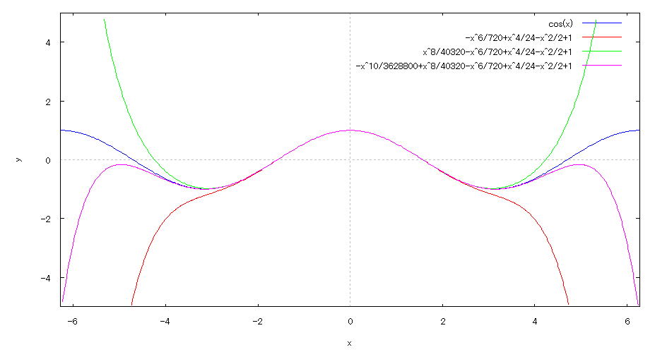 ��How to draw a graph�� �@As in the above input formula , enter all in half-width and press the Shift key and Enter key at the same time. �@ |
| �@�yExample 46�z�@Draw a graph of a 2D explicit function. �mFind a number of real solutions to an equation�n |
�m�P�nEquation �@�@�@�@ �m�Q�nInput formula �@�@�@plot2d([exp(x),3-x^2],[x,-2,2],[y,-1,4]); �m�R�nDrawing result �@�@�@�@�@ 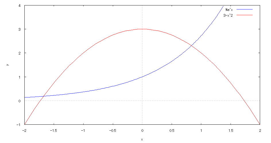 ��How to draw a graph�� �@As in the above input formula , enter all in half-width and press the Shift key and Enter key at the same time. �@Since there are two points of intersection , we know that the equation has two real solutions. �@ |
| �@�yExample 47�z�@Draw a graph of a 2D parameter. �mCircle�FDon't specify the number of divisions�n |
�m�P�nFunction expression �@�@�@�@ �m�Q�nInput formula �@�@�@ plot2d([parametric,cos(t),sin(t)],[t,0,2*%pi]); �m�R�nDrawing result �@�@�@�@�@ 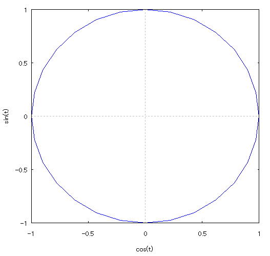 ��How to draw a graph�� �@As in the above input formula , enter all in half-width and press the Shift key and Enter key at the same time. �@ |
| �@�yExample 48�z�@Draw a graph of a 2D parameter. �mCircle�Fspecify 15 divisions�n |
�m�P�nFunction expression �@�@�@�@ �m�Q�nInput formula �@�@�@ plot2d([parametric,cos(t),sin(t)],[t,0,2*%pi],[nticks,15]); �m�R�nDrawing result �@�@�@�@�@ 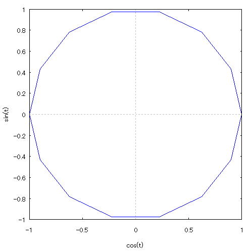 ��How to draw a graph�� �@As in the above input formula , enter all in half-width and press the Shift key and Enter key at the same time. �@ |
| �@�yExample 49�z�@Draw a graph of a 2D parameter. �mCircle�Fspecify 100 divisions�n |
�m�P�nFunction expression �@�@�@�@ �m�Q�nInput formula �@�@�@ plot2d([parametric,cos(t),sin(t)],[t,0,2*%pi],[nticks,100]); �m�R�nDrawing result �@�@�@�@�@ 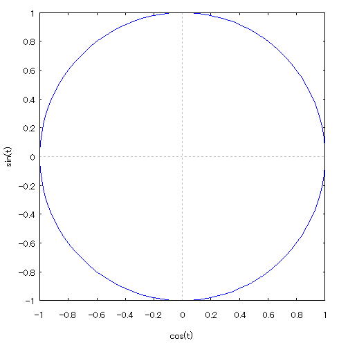 ��How to draw a graph�� �@As in the above input formula , enter all in half-width and press the Shift key and Enter key at the same time. �@ |
| �@�yExample 50�z�@Draw a graph of a 3D explicit function. �mDo not specify the number of divisions�n |
�m�P�nFunction expression �@�@�@�@ �m�Q�nInput formula �@�@�@ plot3d(x^3-3*x*y^2,[x,-1,1],[y,-1,1]); �m�R�nDrawing result �@�@�@�@�@ 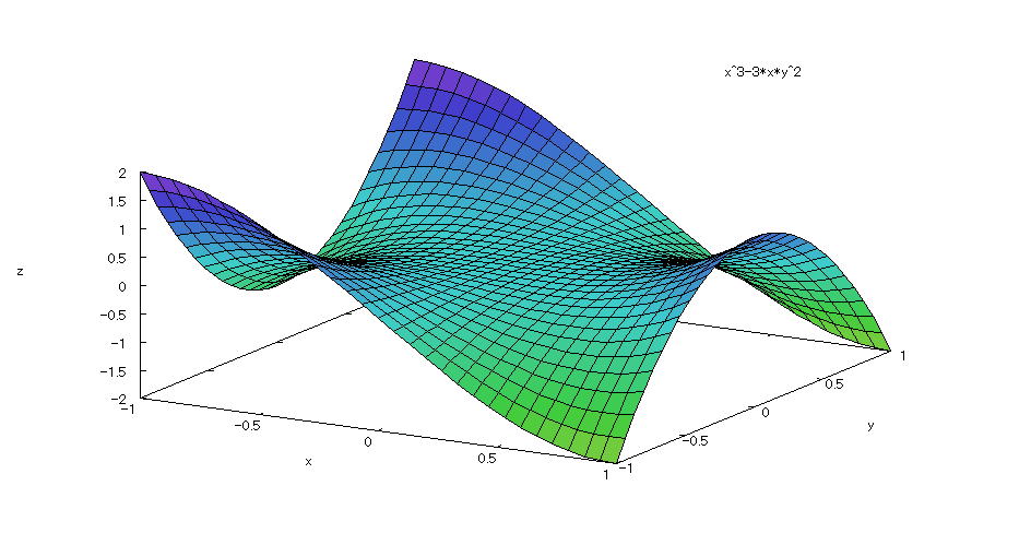 ��How to draw a graph�� �@As in the above input formula , enter all in half-width and press the Shift key and Enter key at the same time. �@ |
| �@�yExample 51�z�@Draw a graph of a 3D explicit function. �mDon't specify the number of divisions�n |
�m�P�nFunction expression �@�@�@�@ �m�Q�nInput formula �@�@�@ plot3d((x^2*y)/(x^4+y^2),[x,-1,1],[y,-1,1]); �m�R�nDrawing result �@�@�@�@�@ 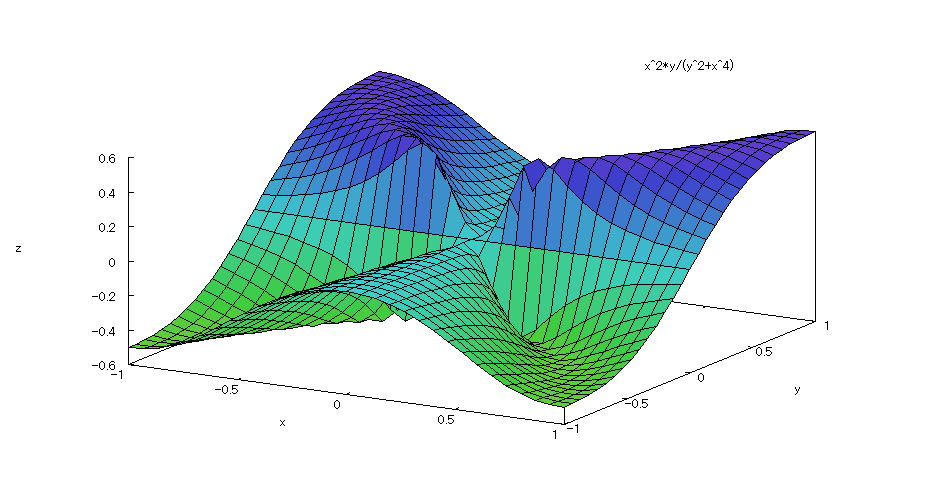 ��How to draw a graph�� �@As in the above input formula , enter all in half-width and press the Shift key and Enter key at the same time. �@ |
| �@�yExample 52�z�@Draw a graph of a 3D explicit function. �mSpecify the number of divisions�n |
�m�P�nFunction expression �@�@�@�@ �m�Q�nInput formula �@�@�@ plot3d((x^2*y)/(x^4+y^2),[x,-1,1],[y,-1,1],[grid,100,100]); �m�R�nDrawing result �@�@�@�@�@ 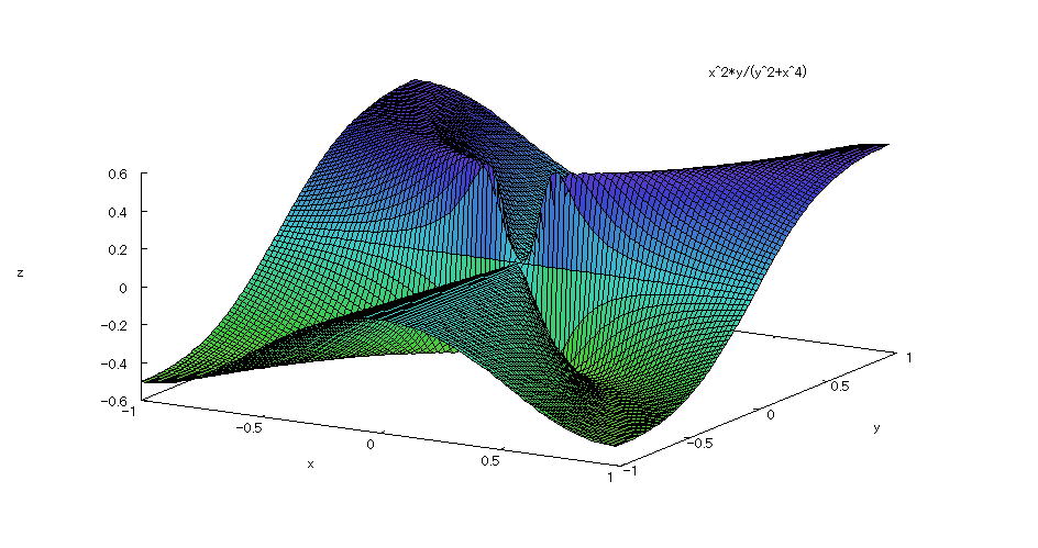 ��How to draw a graph�� �@As in the above input formula , enter all in half-width and press the Shift key and Enter key at the same time. �@ |
| �@�yExample 53�z�@Draw a graph of a 3D parameter. �mSpherical surface�FSpecify the number of division�n |
�m�P�nFunction expression �@�@�@�@ �@�@�@�@�@�O�������Q�A�O�������Q�� �m�Q�nInput formula �@�@�@ plot3d([cos(s)*cos(t),cos(s)*sin(t),sin(s)],[s,0,2*%pi],[t,0,2*%pi],[grid,50,50]); �m�R�nDrawing result �@�@�@�@�@ 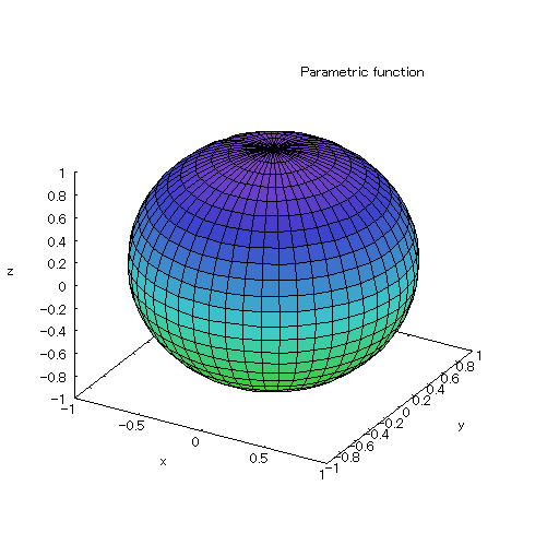 ��How to draw a graph�� �@As in the above input formula , enter all in half-width and press the Shift key and Enter key at the same time. �@ |
| �@�yExample 54�z�@Draw a graph of a 3D parameter. �mAmazing shapes and equations�n |
�m�P�nFunction expression �@�@�@�@ �@�@�@�@�@�@�@�@�@�@�@�@�@�@ �@�@�@�@ �@�@�@�@�@�@�@�@�@�@�@�@�@�@ �@�@�@�@ �@�@�@�@�@�@�@�@�@�@�@�@�@�@�@�@�@�@�@�@�@�@�@�@�@�@�@�@�@�@�@�@�@�@�@�@�@�@�@�@�@�@�@�@�@�O�������Q�A�O�������Q�� �m�Q�nInput formula �@�@�@ plot3d([3*cos(u)+5*cos(3*u)+(3*(cos(u)+5*cos(3*u))*cos(v))/(2*sqrt(234+90*cos(2*u))) �@�@�@ -(3*cos(6*u)*(sin(u)+5*sin(3*u))*sin(v))/(2*sqrt(13+5*cos(2*u))*sqrt(22+5*cos(2*u) �@�@�@ +9*cos(12*u))),3*sin(u)+5*sin(3*u)+(3*cos(v)*(sin(u)+5*sin(3*u)))/(2*sqrt(234+90*cos �@�@ �@(2*u)))+(3*(5*cos(3*u)+cos(5*u)+cos(7*u)+5*cos(9*u))*sin(v))/(4*sqrt(13+5*cos(2*u)) �@�@�@ *sqrt(22+5*cos(2*u)+9*cos(12*u))),3*sin(6*u)-(sqrt(13+5*cos(2*u))*sin(v))/(2*sqrt �@�@ �@(22+5*cos(2*u)+9*cos(12*u)))],[u,0,2*%pi],[v,0,2*%pi],[grid,80,8]); �m�R�nDrawing result �@�@�@�@�@ 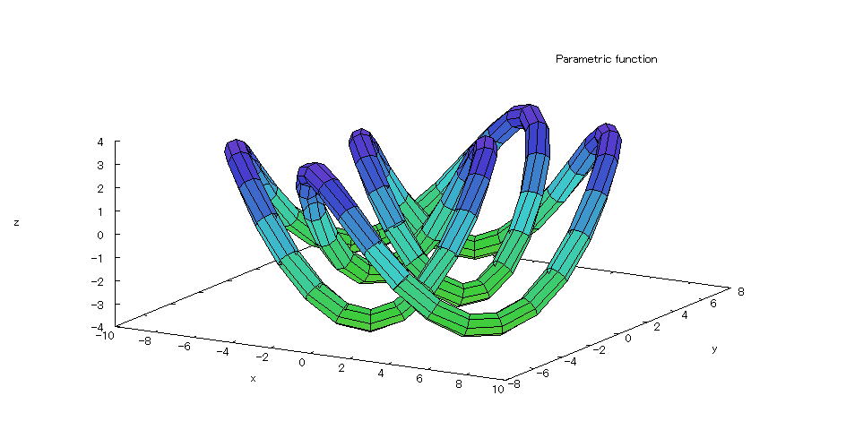 ��How to draw a graph�� �@As in the above input formula , enter all in half-width and press the Shift key and Enter key at the same time. �@ |
| �@�yExample 55�z�@Draw a graph of a 3D parameter. �mRotating body 1�n |
�m�P�nRotating body �@�@�@�@A solid created by rotating the part enclosed by parabola y=x^2 , x=-3 , x=3 , the x-axis around the x-axis. �m�Q�nInput formula �@�@�@ plot3d([t,t^2*cos(s),t^2*sin(s)],[t,-3,3],[s,0,2*%pi]); �m�R�nDrawing result �@�@�@�@�@ 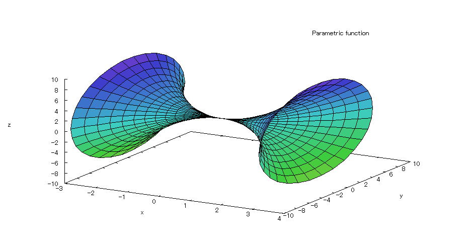 ��How to draw a graph�� �@As in the above input formula , enter all in half-width and press the Shift key and Enter key at the same time. �@ |
| �@�yExample 56�z�@Draw a graph of a 3D parameter. �mRotating body 2�n |
�m�P�nRotating body �@�@�@�@A solid created by rotating the part enclosed by parabola x=�゙ , y=0 , y=9 , the y-axis around the y-axis. �m�Q�nInput formula �@�@�@ plot3d([sqrt(t)*cos(s),t,sqrt(t)*sin(s)],[t,0,9],[s,0,2*%pi]); �m�R�nDrawing result �@�@�@�@�@ 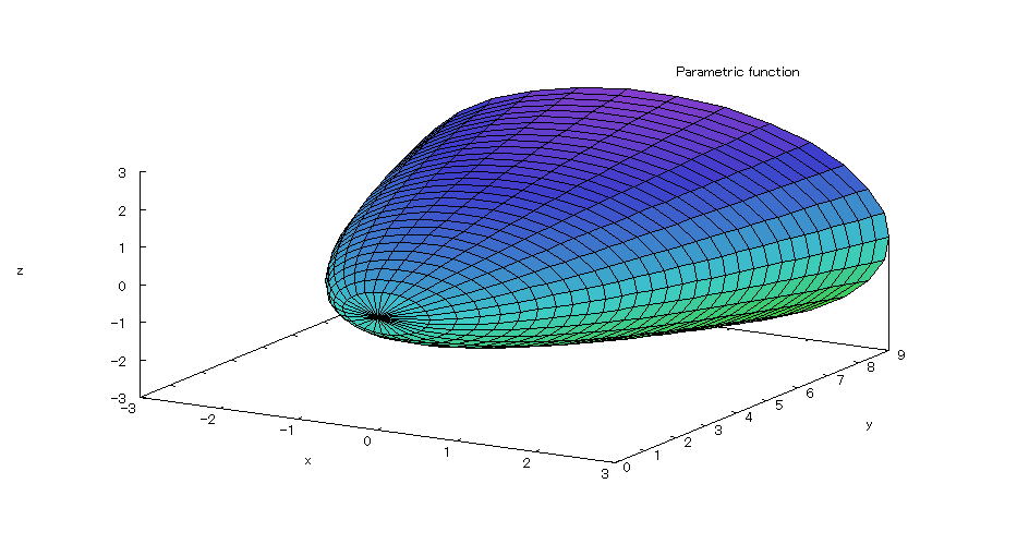 ��How to draw a graph�� �@As in the above input formula , enter all in half-width and press the Shift key and Enter key at the same time. �@ |
| �@�yExample 57�z�@Draw a graph of a 3D parameter. �mRotating body 3�n |
�m�P�nRotating body �@�@�@�@A solid created by rotating the part enclosed by parabola y=x^2-2 , x=-3 , x=3 , the x-axis around the x-axis. �m�Q�nInput formula �@�@�@ plot3d([t,(t^2-2)*cos(s),(t^2-2)*sin(s)],[t,-3,3],[s,0,2*%pi]); �m�R�nDrawing result �@�@�@�@�@ 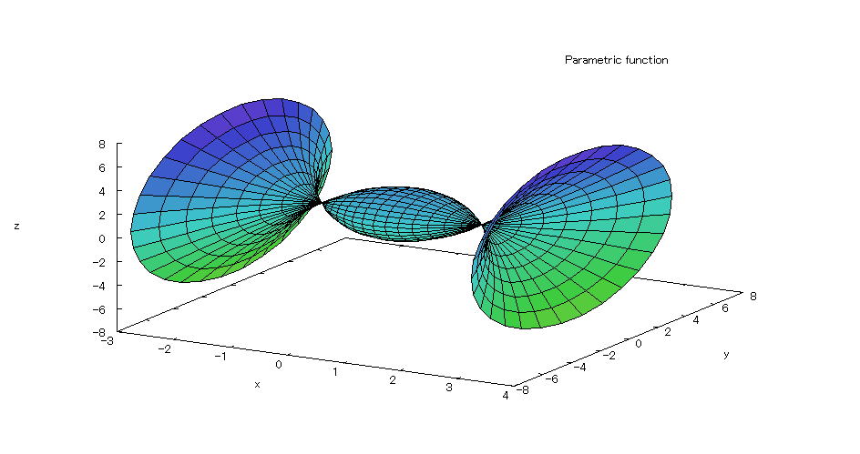 ��How to draw a graph�� �@As in the above input formula , enter all in half-width and press the Shift key and Enter key at the same time. �@ |
| �@�yExample 58�z�@Draw a graph of a 3D parameter. �mRotating body 4�n |
�m�P�nRotating body �@�@�@�@A solid created by rotating the part enclosed by parabola y=x^2+2 , x=-3 , x=3 , the x-axis around the x-axis. �m�Q�nInput formula �@�@�@ plot3d([t,(t^2+2)*cos(s),(t^2+2)*sin(s)],[t,-2,2],[s,0,2*%pi]); �m�R�nDrawing result �@�@�@�@�@ 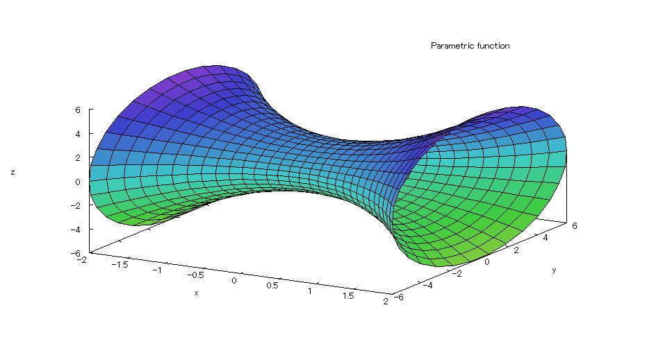 ��How to draw a graph�� �@As in the above input formula , enter all in half-width and press the Shift key and Enter key at the same time. �@ |
| �@�yExample 59�z�@Draw a graph of a 3D parameter. �mRotating body 5�n |
�m�P�nRotating body �@�@�@�@A solid created by rotating circle: x^2+y^2=4 around the x-axis. �m�Q�nInput formula �@�@�@ plot3d([t,sqrt(4-t^2)*cos(s),sqrt(4-t^2)*sin(s)],[t,-2,2],[s,0,2*%pi]); �m�R�nDrawing result �@�@�@�@�@ 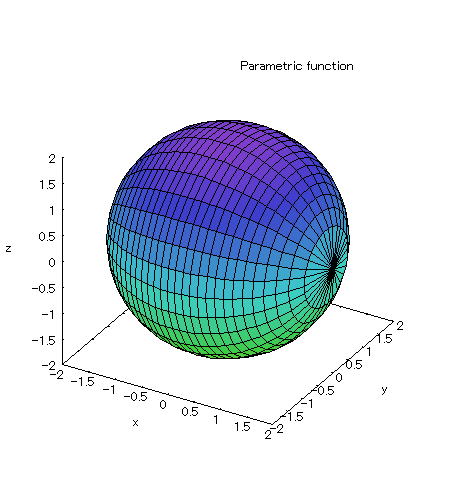 ��How to draw a graph�� �@As in the above input formula , enter all in half-width and press the Shift key and Enter key at the same time. �@ |
| �@�yExample 60�z�@Approximation of expressions by Taylor Expansion �m�������������n |
�m�P�nInput expression for Taylor Expansion of sinx �@�@�@�@taylor(sin(x),x,0,12); �m�Q�nDeployment result �@�@�@ �m�R�nAn input expression that draws the graph of ������������ and its approximation �@�@�@plot2d([sin(x),x-x^3/6+x^5/120-x^7/5040+x^9/362880-x^11/39916800],[x,-10,10],[y,-1.2,1.2]); �m�S�nDrawing result �@�@�@�@�@ 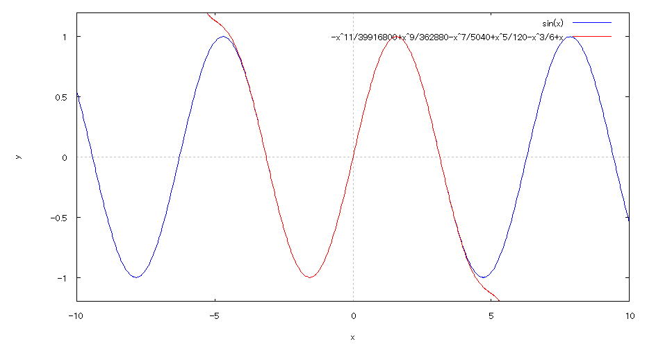 ��How to draw a graph�� �@ As in the input formula in [3] above , enter all in half-width and press the Shift key and Enter key at the same time. �@ |
| �@�yExample 61�z�@Approximation of expressions by Taylor Expansion �m�������������n |
�m�P�nInput expression for Taylor Expansion of cosx �@�@�@�@taylor(cos(x),x,0,12); �m�Q�nDeployment result �@�@�@ �m�R�nAn input expression that draws the graph of ������������ and its aaproximation �@�@�@plot2d([cos(x),1-x^2/2+x^4/24-x^6/720+x^8/40320-x^10/3628800+x^12/479001600] �@�@�@�@�@�@�@�@�@�@�@�@�@�@�@�@�@�@�@�@�@�@�@�@�@�@�@�@�@�@�@�@�@�@�@�@�@�@�@�@�@�@�@�@�@�@�@�@�@,[x,-10,10],[y,-1.2,1.2]); �m�S�nDrawing result �@�@�@�@�@ 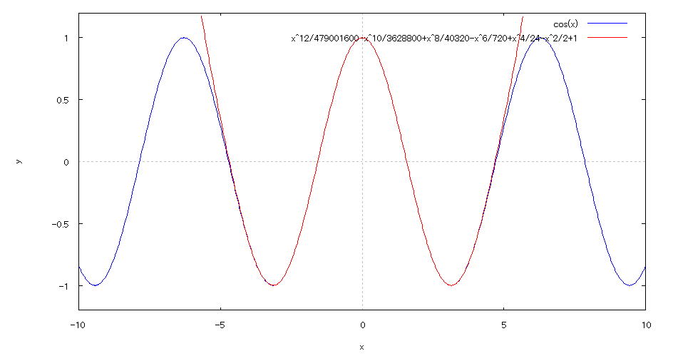 ��How to draw a graph�� �@ As in the input formula in [3] above , enter all in half-width and press the Shift key and Enter key at the same time. �@ |
| �@�yExample 62�z�@Approximation of expressions by Taylor Expansion |
�m�P�nInut expression for Taylor Expansion of e^x �@�@�@�@taylor(exp(x),x,0,6); �m�Q�nDeployment result �@�@�@ 1+x+x^2/2+x^3/6+x^4/24+x^5/120+... �m�R�n An input expression that draws the graph of �@�@�@�@plot2d([exp(x),1+x+x^2/2+x^3/6+x^4/24+x^5/120],[x,-3,3],[y,0,5]); �m�S�nDrawing result �@�@�@�@�@ 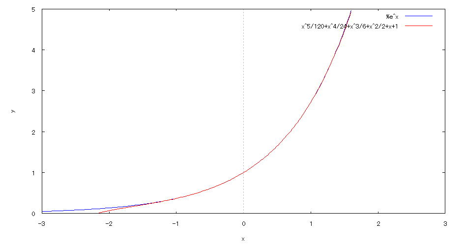 ��How to draw a graph�� �@ As in the input formula in [3] above , enter all in half-width and press the Shift key and Enter key at the same time. �@ |
| �@�yExample 63�z�@Prove Euler's formula |
�m�P�nInput expression for Taylor Expansion of �������� �@�@�@�@taylor(������(x),x,0,12); �m�Q�nTaylor Expansion result of �������� �@�@�@ �m�R�nInput expression for Taylor Expansion of cos�� �@�@�@�@taylor(cos(x),x,0,12); �m�S�nTaylor Expansion result of cos�� �@�@�@�@ �m�T�nInput expression for Taylor Expansion of�@ �@�@�@�@taylor(exp(%i*x),x,0,12); �m�U�nTaylor Expansion result of�@ �@�@�@ �@�@�@�@�|�|�|�B �@�@�@Above , from �@ , �A , �B �@�@�@�@�@ �@�@�@�@�@�@�@�@�@�@�@�@�@�@�@�@�@�@�@ �@�@�@�@�@�@�@�@�� �������� �{ ���������� �@�@�@Therefore , ��How to display the expansion formula�� �@ As in the input formulas in [1] , [3] , [5] above , enter all in half-width and press the Shift key and Enter key at the same time. �@ |
| �@�yProblem 1�z�@How many digits is 2^30 in integer ? However , ������(10�C2)��0.3010. |
| �@This problem always comes up in common logarithms. �@If you teach in the order of �@���A���B���C below , you can make the number of digits more specific. �@Display 2^30 , 2^50 , 2^100 , 3^30 , 3^50 , and 3^100 computed by �l���������� and count the number of digits. �ATeach how to find the number of digits by using common rogarithms. �BFind the number of digits in 2^30 , 2^50 , 2^100 , 3^30 , 3^50 , and 3^100 using common logarithms and comfirm that it matches the number of digits you just counted. �CTouching on how to count large numbers. Below are the results caluculated by Maxima. �@2^30��1073741824 �@2^50��1125899906842624 �@2^100��1267650600228229401496703205376 �@3^30��205891132094649 �@3^50��717897987691852588770249 �@3^100��515377520732011331036461129765621272702107522001 ��How to use "�l����������"�� �@For example , to calculate 2^30 �@Enter 2^30�@in half-width , and press the Shift key and Enter key at the same time. |
| �@�yProblem 2�z�@Expand �i���{���j^3�@and�@�i���{���{���j^2�@ |
| �@Expanding �i���{���j^3�@or�@�i���{���{���j^2�@doesn't surprise you much. �@I wondered if it would be possible to have a class that surprises and impresses students by having Maxima calculate and display the expansion of �i���{���j^50 and �i���{���{���j^20 in the introduction of the expansion of equations. Below is the result of expansion by Maxima �@�@�i���{���j^50 �@��b^50+50*a*b^49+1225*a^2*b^48+19600*a^3*b^47+230300*a^4*b^46+2118760*a^5*b^45 �@�@+15890700*a^6*b^44+99884400*a^7*b^43+536878650*a^8*b^42+2505433700*a^9*b^41 �@�@+10272278170*a^10*b^40+37353738800*a^11*b^39+121399651100*a^12*b^38 �@�@+354860518600*a^13*b^37+937845656300*a^14*b^36+2250829575120*a^15*b^35 �@�@+4923689695575*a^16*b^34+9847379391150*a^17*b^33+18053528883775*a^18*b^32 �@�@+30405943383200*a^19*b^31+47129212243960*a^20*b^30+67327446062800*a^21*b^29 �@�@+88749815264600*a^22*b^28+108043253365600*a^23*b^27+121548660036300*a^24*b^26 �@�@+126410606437752*a^25*b^25+121548660036300*a^26*b^24+108043253365600*a^27*b^23 �@�@+88749815264600*a^28*b^22+67327446062800*a^29*b^21+47129212243960*a^30*b^20 �@�@+30405943383200*a^31*b^19+18053528883775*a^32*b^18+9847379391150*a^33*b^17 �@�@+4923689695575*a^34*b^16+2250829575120*a^35*b^15+937845656300*a^36*b^14 �@�@+354860518600*a^37*b^13+121399651100*a^38*b^12+37353738800*a^39*b^11 �@�@+10272278170*a^40*b^10+2505433700*a^41*b^9+536878650*a^42*b^8+99884400*a^43*b^7 �@�@+15890700*a^44*b^6+2118760*a^45*b^5+230300*a^46*b^4+19600*a^47*b^3+1225*a^48*b^2 �@�@+50*a^49*b+a^50 �@�@�i���{���{���j^20 �@��c^20+20*b*c^19+20*a*c^19+190*b^2*c^18+380*a*b*c^18+190*a^2*c^18+1140*b^3*c^17 �@�@+3420*a*b^2*c^17+3420*a^2*b*c^17+1140*a^3*c^17+4845*b^4*c^16+19380*a*b^3*c^16 �@�@+29070*a^2*b^2*c^16+19380*a^3*b*c^16+4845*a^4*c^16+15504*b^5*c^15+77520*a*b^4*c^15 �@�@+155040*a^2*b^3*c^15+155040*a^3*b^2*c^15+77520*a^4*b*c^15+15504*a^5*c^15 �@�@+38760*b^6*c^14+232560*a*b^5*c^14+581400*a^2*b^4*c^14+775200*a^3*b^3*c^14 �@�@+581400*a^4*b^2*c^14+232560*a^5*b*c^14+38760*a^6*c^14+77520*b^7*c^13 �@�@+542640*a*b^6*c^13+1627920*a^2*b^5*c^13+2713200*a^3*b^4*c^13+2713200*a^4*b^3*c^13 �@�@+1627920*a^5*b^2*c^13+542640*a^6*b*c^13+77520*a^7*c^13+125970*b^8*c^12 �@�@+1007760*a*b^7*c^12+3527160*a^2*b^6*c^12+7054320*a^3*b^5*c^12 �@�@+8817900*a^4*b^4*c^12+7054320*a^5*b^3*c^12+3527160*a^6*b^2*c^12 �@�@+1007760*a^7*b*c^12+125970*a^8*c^12+167960*b^9*c^11+1511640*a*b^8*c^11 �@�@+6046560*a^2*b^7*c^11+14108640*a^3*b^6*c^11+21162960*a^4*b^5*c^11 �@�@+21162960*a^5*b^4*c^11+14108640*a^6*b^3*c^11+6046560*a^7*b^2*c^11 �@�@+1511640*a^8*b*c^11+167960*a^9*c^11+184756*b^10*c^10+1847560*a*b^9*c^10 �@�@+8314020*a^2*b^8*c^10+22170720*a^3*b^7*c^10+38798760*a^4*b^6*c^10 �@�@+46558512*a^5*b^5*c^10+38798760*a^6*b^4*c^10+22170720*a^7*b^3*c^10 �@�@+8314020*a^8*b^2*c^10+1847560*a^9*b*c^10+184756*a^10*c^10+167960*b^11*c^9 �@�@+1847560*a*b^10*c^9+9237800*a^2*b^9*c^9+27713400*a^3*b^8*c^9 �@�@+55426800*a^4*b^7*c^9+77597520*a^5*b^6*c^9+77597520*a^6*b^5*c^9 �@�@+55426800*a^7*b^4*c^9+27713400*a^8*b^3*c^9+9237800*a^9*b^2*c^9 �@�@+1847560*a^10*b*c^9+167960*a^11*c^9+125970*b^12*c^8+1511640*a*b^11*c^8 �@�@+8314020*a^2*b^10*c^8+27713400*a^3*b^9*c^8+62355150*a^4*b^8*c^8 �@�@+99768240*a^5*b^7*c^8+116396280*a^6*b^6*c^8+99768240*a^7*b^5*c^8 �@�@+62355150*a^8*b^4*c^8+27713400*a^9*b^3*c^8+8314020*a^10*b^2*c^8 �@�@+1511640*a^11*b*c^8+125970*a^12*c^8+77520*b^13*c^7+1007760*a*b^12*c^7 �@�@+6046560*a^2*b^11*c^7+22170720*a^3*b^10*c^7+55426800*a^4*b^9*c^7 �@�@+99768240*a^5*b^8*c^7+133024320*a^6*b^7*c^7+133024320*a^7*b^6*c^7 �@�@+99768240*a^8*b^5*c^7+55426800*a^9*b^4*c^7+22170720*a^10*b^3*c^7 �@�@+6046560*a^11*b^2*c^7+1007760*a^12*b*c^7+77520*a^13*c^7+38760*b^14*c^6 �@�@+542640*a*b^13*c^6+3527160*a^2*b^12*c^6+14108640*a^3*b^11*c^6 �@�@+38798760*a^4*b^10*c^6+77597520*a^5*b^9*c^6+116396280*a^6*b^8*c^6 �@�@+133024320*a^7*b^7*c^6+116396280*a^8*b^6*c^6+77597520*a^9*b^5*c^6 �@�@+38798760*a^10*b^4*c^6+14108640*a^11*b^3*c^6+3527160*a^12*b^2*c^6 �@�@+542640*a^13*b*c^6+38760*a^14*c^6+15504*b^15*c^5+232560*a*b^14*c^5 �@�@+1627920*a^2*b^13*c^5+7054320*a^3*b^12*c^5+21162960*a^4*b^11*c^5 �@�@+46558512*a^5*b^10*c^5+77597520*a^6*b^9*c^5+99768240*a^7*b^8*c^5 �@�@+99768240*a^8*b^7*c^5+77597520*a^9*b^6*c^5+46558512*a^10*b^5*c^5 �@�@+21162960*a^11*b^4*c^5+7054320*a^12*b^3*c^5+1627920*a^13*b^2*c^5 �@�@+232560*a^14*b*c^5+15504*a^15*c^5+4845*b^16*c^4+77520*a*b^15*c^4 �@�@+581400*a^2*b^14*c^4+2713200*a^3*b^13*c^4+8817900*a^4*b^12*c^4 �@�@+21162960*a^5*b^11*c^4+38798760*a^6*b^10*c^4+55426800*a^7*b^9*c^4 �@�@+62355150*a^8*b^8*c^4+55426800*a^9*b^7*c^4+38798760*a^10*b^6*c^4 �@�@+21162960*a^11*b^5*c^4+8817900*a^12*b^4*c^4+2713200*a^13*b^3*c^4 �@�@+581400*a^14*b^2*c^4+77520*a^15*b*c^4+4845*a^16*c^4+1140*b^17*c^3 �@�@+19380*a*b^16*c^3+155040*a^2*b^15*c^3+775200*a^3*b^14*c^3 �@�@+2713200*a^4*b^13*c^3+7054320*a^5*b^12*c^3+14108640*a^6*b^11*c^3 �@�@+22170720*a^7*b^10*c^3+27713400*a^8*b^9*c^3+27713400*a^9*b^8*c^3 �@�@+22170720*a^10*b^7*c^3+14108640*a^11*b^6*c^3+7054320*a^12*b^5*c^3 �@�@+2713200*a^13*b^4*c^3+775200*a^14*b^3*c^3+155040*a^15*b^2*c^3 �@�@+19380*a^16*b*c^3+1140*a^17*c^3+190*b^18*c^2+3420*a*b^17*c^2 �@�@+29070*a^2*b^16*c^2+155040*a^3*b^15*c^2+581400*a^4*b^14*c^2 �@�@+1627920*a^5*b^13*c^2+3527160*a^6*b^12*c^2+6046560*a^7*b^11*c^2 �@�@+8314020*a^8*b^10*c^2+9237800*a^9*b^9*c^2+8314020*a^10*b^8*c^2 �@�@+6046560*a^11*b^7*c^2+3527160*a^12*b^6*c^2+1627920*a^13*b^5*c^2 �@�@+581400*a^14*b^4*c^2+155040*a^15*b^3*c^2+29070*a^16*b^2*c^2 �@�@+3420*a^17*b*c^2+190*a^18*c^2+20*b^19*c+380*a*b^18*c+3420*a^2*b^17*c �@�@+19380*a^3*b^16*c+77520*a^4*b^15*c+232560*a^5*b^14*c+542640*a^6*b^13*c �@�@+1007760*a^7*b^12*c+1511640*a^8*b^11*c+1847560*a^9*b^10*c �@�@+1847560*a^10*b^9*c+1511640*a^11*b^8*c+1007760*a^12*b^7*c �@�@+542640*a^13*b^6*c+232560*a^14*b^5*c+77520*a^15*b^4*c+19380*a^16*b^3*c �@�@+3420*a^17*b^2*c+380*a^18*b*c+20*a^19*c+b^20+20*a*b^19+190*a^2*b^18 �@�@+1140*a^3*b^17+4845*a^4*b^16+15504*a^5*b^15+38760*a^6*b^14 �@�@+77520*a^7*b^13+125970*a^8*b^12+167960*a^9*b^11+184756*a^10*b^10 �@�@+167960*a^11*b^9+125970*a^12*b^8+77520*a^13*b^7+38760*a^14*b^6 �@�@+15504*a^15*b^5+4845*a^16*b^4+1140*a^17*b^3+190*a^18*b^2+20*a^19*b+a^20 ��How to use "Maxima"�� �@For example , when expanding (a+b)^50 �@Enter expand((a+b)^50)�@in half-width , and press the Shift key and Enter key at the same time. |
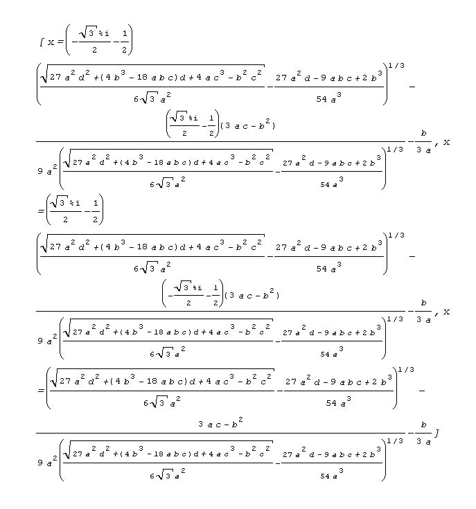
| �@�yProblem 3�z�@Solve the higher equation ��^3�{�Q��^2�{�Q���{�P���O. |
| �@The high-level equation handled in high school is a form that can be solved
by using factor decomposition or the like , or can be solved as x^2=t or
the like. �@Solve the cubic equation ax^3+bx^2+cx+d=0 in "Maxima". Then the formula of the cubic equation is displayed. Will the students be surprised and impressed ? �@Also , if you solve the cubic equation ��^3�|�U���|�P�O���O�@, and the quartic equation ��^4�{�R��^3�|�P�W��^2�{�U���|�T���O�@using Maxima and display them , the complexity of the solution should surprise the students. ��How to use "�l����������"�� �@For example , when solving ax^3+bx^2+cx+d=0 �@Enter solve(��*��^3�{��*��^2�{��*���{�����O,x)�@in half-width , press the Shift key and Enter key at the same time. |
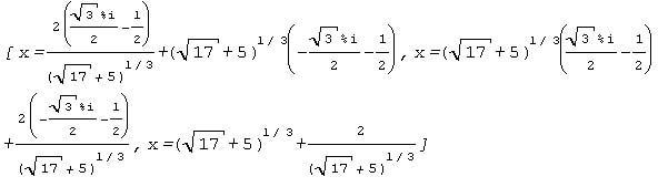
| �@The result of letting "Maxima"�@solve a cubic equation ����^3�{����^2�{�����{�����O |
 |
| �@The result of letting "Maxima" solve a cubic equation �@��^3�|�U���|�P�O���O |
 |
| �@�yProblem 4�z�@Factor �����|���{���|�P |
| �@This is a problem of cleaning up and factoring for one character. �@If we let Maxima solve more complex factorizations and display them , I wondered if it would be possible to create a class that surprises and impresses the students. �@Students would be surprised if�@(���{���{��)(�����{�����{����)�|������ , (���|��)^3�{(���|��)^3�{(���|��)^3 , ��^3�{��^3�{��^3�|�R������ , and (���{��)(���{��)(���{��)�{������ were factored instantly , using Maxima displayed. Below is the result of following with "Maxima" �@(a+b+c)(bc+ca+ab)-abc = (b+a)(c+a)(c+b) �@(b-c)^3+(c-a)^3+(a-b)^3 = 3(b-a)(c-a)(c-b) �@a^3+b^3+c^3-3*a*b*c = (c+b+a)(c^2-b*c-a*c+b^2-a*b+a^2) �@(b+c)(c+a)(a+b)+abc = (c+b+a)(bc+ac+ab) ��How to use "Maxima"�� �@For example , when factoring (a+b+c)(bc+ca+ab)-abc �@ �@Enter factor((a+b+c)*(b*c+c*a+a*b)-a*b*c)�@in half-width , and press the Shift key and Enter key at the same time. |
| �@�yProblem 5�z�@Differentiate (���{�V��^2)^(1/3).�@ |
| �@I wonder if I could create a class that surprise and impress students
by searching for more complex expressions in workbooks and using "Maxima"
to differentiate them and display them. Below is the result of differentiating with "Maxima" �@{(���{�V��^2)^(1/3)}�f = (14*x+1)/(3*(7*x^2+x)^(2/3)) ��How to use "�l����������"�� �@For example , when differentiating (���{�V��^2)^(1/3) �@Enter diff((x+7*x^2)^(1/3), x)�@in half-width , and press the Shift key and Enter key at the same time. |
| �@�yProblem 6�z�@Integrate ��(�P�{�T��)�@ |
| �@I wonder if I could create a class that surprises and impresses by searching
for more complex expressions in workbooks and using "Maxima"
to integrate them and display them. Below is the result of integrating with "Maxima". ���(�P�{�T��)���� = (2*(5*x+1)^(3/2))/15 ��How to use "�l����������"�� �@For example , when integrating�@��(�P�{�T��) �@Enter integrate(sqrt(1+5*x) , x)�@in half-width , and press the Shift key and Enter key at the same time. |
| �@Formula manipulation software "Maxima" | �@Formula manipulation software "wx�l����������" |
| �@Click on the formula manipulation software "�����l����������" above to open Maxima's official website. �@Click Download on the left menue of this wxMaxima official site. �@Next , click Sourceforge download page. �@And , click Maxima Windows. �@Furthermore , click 5.26.0-Windows. �@Then , ckick maxima-5.26.0.exe to download "maxima 5.26.0.exe". �@Double-click "maxima-5.26.0.exe" downloaded to launch the Maxima installer. �@After that , follow the instructions on the screen to install. However , 5.26.0 in "maxima-5.26.0.exe" represents the version. (2/12/2012) |
| �@Since the icon of "wxMaxima" is created on the desktop , double-click it to start "Maxima". |
| �@You can download a Maxima data file "MSample.wxm" containing
all the sample programs shown on this website. �@Click the data file "MSamp.lzh" and save it to your desktop or other location. �@Unzip the downloaded file "MSamp.lzh" , put the cursor on the input expression you want to excute , and press the Shift key and Enter key at the same time to excute it. Of course , "Maxima" must be installed before that. |
| Data file "MSamp.wxm" |